This is to do exactly same thing that I did in the feedforwardet tutorial, but using different neural network called CNN(Convolutional Neural Network). In fact, this is just to do a simple thing in a fancy looking way -:). This tutorial is also for introducing the overall syntax for bulding / training CNN and the training dataset itself is pretty much oversimplified and may not be much sense in practice, but I think this tutorial would show you some basic/critical component of CNN and give you a big picture on how a CNN can be built and trained.
I think you may find many of CNN examples in tech documents or in youTube video and they may be more realistic, but most of those examples tend to be too complicated for the beginners to grasp the meaning out of it. Of course, those CNNs which are really used in the industry (like image recoginition system) is much more complicated than those open examples. That's why I decided to write an example with the simplest CNN so that even the begginners can easily understand the whole structure without difficulties
- CNN - one Convolution Layer and one Fully Connected layer
- Step 1 : Preparation of Labeled Image
- Step 2 : Read the labeled image and construct the training data
- Step 3 : Construct a Neural Net
- Step 4 : Configure the detailed network Parameter
- Step 5 : Analyze the network
- Step 6 : Train the network
- Step 7 : Test the network
- CNN - three Convolution Layer and one Fully Connected layer
CNN - one Convolution Layer and one Fully Connected layer
Step 1 : Preparation of Labeled Image
To apply a neural net for digit classification (a type of image classification application), first you need to prepare a set of labeled image. This can be a good example of various data preparation that I mentioned in what they do page. There can be various way to prepare the labeled data for the training, but the way I take is as follows.
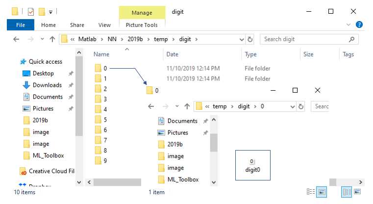
i) First, I created 10 folders with the folder name matching the label for the images that are stored in the folder. i.e, I created 10 folders with name 0,1,2,3,4,5,6,7,8,9 as shown below.
ii) Then, I put the images with numbers written on it.
NOTE 1 : For simplicity, I have created all the image files with the same size. In real situation, you may get all of these images with different size.
NOTE 2 : To reduce the size of input layer and hidden layers I have written numbers in a very small image (just 10 x 10 pixels).
NOTE 3 : As another measure for simplification of data preparation, I put only single image for each label. It mean that this network would not work very well in real life situation with a lot of variations of image.
Step 2 : Read the labeled image and construct the training data
At this step, I will read (load) all the image files and store them into a variable called imds (image data set). Basically this is same logic as in step 2 of feedforwardnet digit classifier tutorial. But in the feedforwardnet tutorial, I read all the images one by one and add it into a vector using in the for loop, but in this tutorial I will use a special function called imageDatastor() function which basically read all the image files in every folders and save them into a variable without using for or while loop (of course, internally within this function there will be some loops running to read the files one by one, but at least we (as users) don't need to care about those loops).
digitDatasetPath = sprintf('%s\\temp\\digit',pwd);
imds = imageDatastore(digitDatasetPath, ...
'IncludeSubfolders',true,'LabelSource','foldernames');
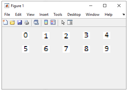
Then just for checking the images, I would plot some of the images (in this tutorial I would plot all the images because there are not many) as follows.
for i = 1:10
subplot(4,5,i);
imshow(imds.Files{i},'InitialMagnification','fit');
end
set(gcf,'Position',[100 100 400 200]);
Step 3 : Construct a Neural Net
Now I would construct a CNN with a very simple structure (basically one convolution layer and one output layer as shown below. This concept is very similar to Pytorch nn.Linear(). Just put all the network components in equance from top to the bottom. Here, the variable name 'layer' is user defined variable meaning you can use any name, but imageImputLayer(), convolutional2dLayer(), batchNormalizationLayer, reluLayer, fullyConnectedLayer(), softmaxLayer, classificationLayer are all the built-in function of Matlab Machine Learning toolbox. So you would get errors with even single spelling or case mistake.
layers = [
imageInputLayer([10 10 3]) % image size = 10 x 10, image layer = 3 (three color image)
convolution2dLayer(3,8,'Padding','same') % filter size = 3 x 3, number of filters = 8, Padding = no,
batchNormalizationLayer % perform batchNormalization for the convolved data
reluLayer % use ReLu as the activation (transfer) function of this convolution2dLayer networ
fullyConnectedLayer(10) % Construct a fullyConnected Network (a kind of feedforwardnet)
% with the output size = 10. Input size of this network is automatically determined
% by the previous layer (i.e, imageInputLayer in this case)
softmaxLayer % use softmax function as the activation function of the fullyConnectedLayer
classificationLayer % return the classification output
];
Step 4 : Configure the detailed network Parameter
Now let's configure the detailed parameters of the network. In CNN case, it is to define various training related parameters as below. I would not go through each parameters... just to let you know that you can control various aspect of training the CNN in this way. For the details, refer to Machine Learning toolbox documents.
options = trainingOptions('sgdm', ...
'InitialLearnRate',0.01, ...
'MaxEpochs',10, ...
'Shuffle','every-epoch', ...
'ValidationData',imdsValidation, ...
'ValidationFrequency',30, ...
'Verbose',false, ...
'Plots', ...
'training-progress');
Step 5 : Analyze the network
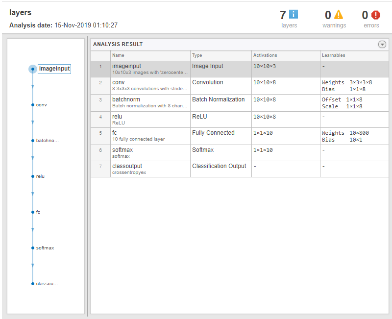
This is not the mandatory but very often (actually almost always) the structure of a CNN tend to be very complicated. So it would be good if there is a way to describe the structure of the network in nicely designed table as shown below.
Just the single function call shown below will show you a nicely written table as below.
analyzeNetwork(layers);
Step 6 : Train the network
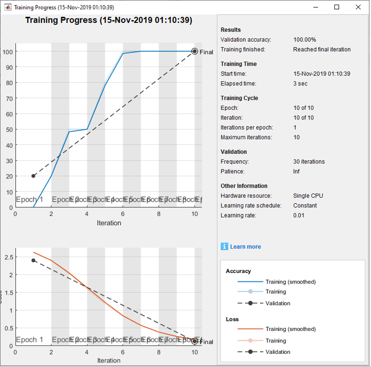
Once you define all the details on network structure and training parameters, training itself can be done as simply as possible giving a real time graph as below.
net = trainNetwork(imdsTrain,layers,options);
Step 7 : Test the network
Now you can validate (test) the trained network as shown below.
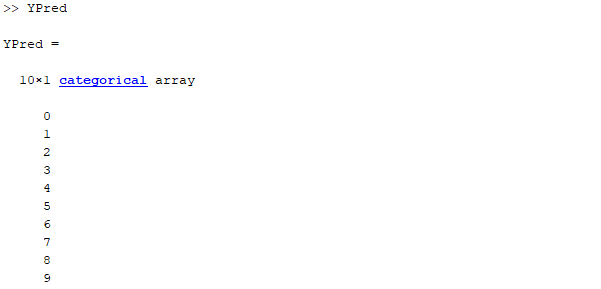
YPred = classify(net,imdsValidation)
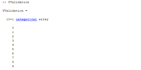
YValidation = imdsValidation.Labels
accuracy = sum(YPred == YValidation)/numel(YValidation)
Then, print out the result and see if it is as you expcted.
|
% load the training/testing image and store them into variables
digitDatasetPath = sprintf('%s\\temp\\digit',pwd); imds = imageDatastore(digitDatasetPath, ... 'IncludeSubfolders',true,'LabelSource','foldernames');
%plot the image for check;
for i = 1:10 subplot(4,5,i); imshow(imds.Files{i},'InitialMagnification','fit'); end set(gcf,'Position',[100 100 400 200]);
% split the image data into training and validation data imdsTrain = imds; imdsValidation = imds;
% Construct (define) a CNN layers = [ imageInputLayer([10 10 3])
convolution2dLayer(3,8,'Padding','same') batchNormalizationLayer reluLayer
fullyConnectedLayer(10) softmaxLayer classificationLayer];
% define a training options options = trainingOptions('sgdm', ... 'InitialLearnRate',0.01, ... 'MaxEpochs',10, ... 'Shuffle','every-epoch', ... 'ValidationData',imdsValidation, ... 'ValidationFrequency',30, ... 'Verbose',false, ... 'Plots','training-progress');
% print out network structure analyzeNetwork(layers);
% train the network net = trainNetwork(imdsTrain,layers,options);
% test the network YPred = classify(net,imdsValidation) YValidation = imdsValidation.Labels
% check test accuracy accuracy = sum(YPred == YValidation)/numel(YValidation) |
CNN - three Convolution Layer and one Fully Connected layer
Step 1 : Preparation of Labeled Image
This is exactly same procedure as in previous example.
Step 2 : Read the labeled image and construct the training data
This is exactly same procedure as in previous example.
Step 3 : Construct a Neural Net
Now let's construct a CNN for the problem. The network that created is as follows. If you remember the network structure in previous section, you would notice that the first 4 lines and the last three lines are exactly same as the one in previous section. The 8 lines in between are the one that I inserted. Why ? No specific reason. I just wanted to make the network just a little bit more complicated -:) and see how it works. You would also notice that there is a component that you didn't see in previous section. It is maxPooling2dLayer(). As the name implies this is the layer that perform 'Pooling' based on max value (For now, I assume that you understand the concept of Pooling. I will try to write the concept of the basic components of CNN in separate page or you can just google the concept).
layers = [
imageInputLayer([10 10 3])
convolution2dLayer(3,8,'Padding','same')
batchNormalizationLayer
reluLayer
maxPooling2dLayer(2,'Stride',2)
convolution2dLayer(3,16,'Padding','same')
batchNormalizationLayer
reluLayer
maxPooling2dLayer(2,'Stride',2)
convolution2dLayer(3,32,'Padding','same')
batchNormalizationLayer
reluLayer
fullyConnectedLayer(10)
softmaxLayer
classificationLayer];
Step 4 : Configure the detailed network Parameter
Now let's configure the detailed parameters of the network. In CNN case, it is to define various training related parameters as below. I would not go through each parameters... just to let you know that you can control various aspect of training the CNN in this way. For the details, refer to Machine Learning toolbox documents.
options = trainingOptions('sgdm', ...
'InitialLearnRate',0.01, ...
'MaxEpochs',10, ...
'Shuffle','every-epoch', ...
'ValidationData',imdsValidation, ...
'ValidationFrequency',30, ...
'Verbose',false, ...
'Plots','training-progress');
Step 5 : Analyze the network
This is not the mandatory but very often (actually almost always) the structure of a CNN tend to be very complicated. So it would be good if there is a way to describe the structure of the network in nicely designed table as shown below.
Just the single function call shown below will show you a nicely written table as below.
analyzeNetwork(layers);
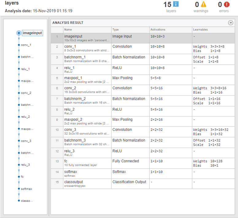
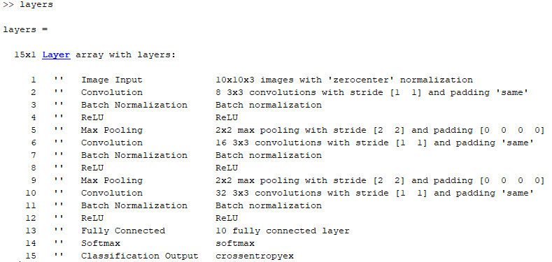
or you can just print out the variable that stores the network and you will get the structural information of the network in text format as shown below.
Step 6 : Train the network
Once you define all the details on network structure and training parameters, training itself can be done as simply as possible giving a real time graph as below.
net = trainNetwork(imdsTrain,layers,options);

Step 7 : Test the network
Now you can validate (test) the trained network as shown below.
YPred = classify(net,imdsValidation)
YValidation = imdsValidation.Labels
accuracy = sum(YPred == YValidation)/numel(YValidation)
Then, print out the result and see if it is as you expcted.
|
% Load all the image and store them to a variable
digitDatasetPath = sprintf('%s\\temp\\digit',pwd); imds = imageDatastore(digitDatasetPath, ... 'IncludeSubfolders',true,'LabelSource','foldernames');
% plot some of the image for check
for i = 1:10 subplot(4,5,i); imshow(imds.Files{i},'InitialMagnification','fit'); end set(gcf,'Position',[100 100 400 200]);
% split the image set into training and validation group
imdsTrain = imds; imdsValidation = imds;
% define the network structure
layers = [ imageInputLayer([10 10 3])
convolution2dLayer(3,8,'Padding','same') batchNormalizationLayer reluLayer
maxPooling2dLayer(2,'Stride',2)
convolution2dLayer(3,16,'Padding','same') batchNormalizationLayer reluLayer
maxPooling2dLayer(2,'Stride',2)
convolution2dLayer(3,32,'Padding','same') batchNormalizationLayer reluLayer
fullyConnectedLayer(10) softmaxLayer classificationLayer];
% define the training parameters
options = trainingOptions('sgdm', ... 'InitialLearnRate',0.01, ... 'MaxEpochs',10, ... 'Shuffle','every-epoch', ... 'ValidationData',imdsValidation, ... 'ValidationFrequency',30, ... 'Verbose',false, ... 'Plots','training-progress');
% analyze overal network structure
analyzeNetwork(layers);
% perform training
net = trainNetwork(imdsTrain,layers,options);
% validate (test) the trained network
YPred = classify(net,imdsValidation); YValidation = imdsValidation.Labels;
% check the accuracy
accuracy = sum(YPred == YValidation)/numel(YValidation) |
Next Step :