This page is to show how to implement single perceptron using Matlab Deep Learning Toolbox. This is not about explaining on theory / mathematical procedure of Perceptron. For mathematical background of single perceptron, I wrote a separate page for it. If you are not familiar with exact mechanism on how the perceptron works, I would recommend you to read the theory part first and it would be even better if you pick a simple example and go through each steps by hands (For this kind of practice problem, try AND, OR, NOR table implementation with single perceptron).
Now you think you are quite confident about how single perceptron works ? Then, let's see how you can build the simplest neural network with Matlab toolbox.
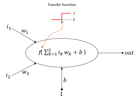
The network we are trying to build is a single neuron (perceptron) as shown below.
Now let's look into some key commands in Matlab Deep Learning package that are used to implement this.
The first command to look at is as follows.
net = perceptron;
This creates a perceptron but the exact structure (e.g, number of input etc) is not determined yet. The number of input and output is configured by following function.
net = configure(net,[0;0],[0]);
The dimension of the first matrix(vector) is 2 x 1. It mean that the input to this nework is 2x1 vector. That is, the number of inputs to this network is 2. The specific number in this vector does not matter much because the values of the inputs will be initialized next step.
The dimension of the second matrix(vector) is 1 x 1. It mean that the output of this network is 1 x 1. That is, the number of output of this betwork is 1.
Now we initialize each component of the network(perceptron) as follows.
net.b{1} = [0];
this initialize the bias of the first layer of the network(the number '1' in {1} indicates 'first layer'). In case of Single Perceptron, the number of layer is only one and the number of neurons in the layer is also only one. So the bias is initialized by 1x1 matrix.
Then initialize the weight vector and it is done as follows.
w = [1 -0.8];
net.IW{1,1} = w;
IW{1,1} indicates the input weights of the first layer, first neuron. In this example, we have two inputs to the single neuron. So this is initialized by 2x1 vector. Note that the dimension of this matrix should match the dimension of the first matrix in configure() function should match, otherwise you will get error.
Now we completed the network creation and initialization. Next step is to train the network using a set of training data. This is the most complicated (and hard to understand) part in neural network implementation, but this can be done by single function call as shown below. In my example, I provide only four traning data, but it doesn't mean that the train() function perform only 4 iterations to train. It automatically(and randomly) picks the specific data from the provided set as many as possible until the training complete.
net = train(net,pList,tList);
NOTE : this train() function can be one of the biggest advantage of Matlab Deep Learning Toolbox comparing to PyTorch or Tensorflow. In PyTorch and TensorFlow, you have to define your own update rule(back propogation rule) and define a loop that performs the train and update weight & bias.
Transfer Functions
By default, the hardlimit() type of function is used as the transfer function, but you can apply a various different transfer function to each perceptron if you like by using following command.
NET.layers{i}.transferFcn
If the network is a single perceptron, you can change the transfer function as in the following example.
net.layers{1}.transferFcn = 'logsig'.
There are many different types of transfer functions defined in Deep Learning toolbox as listed below.
- compet - Competitive transfer function.
- elliotsig - Elliot sigmoid transfer function.
- hardlim - Positive hard limit transfer function.
- hardlims - Symmetric hard limit transfer function.
- logsig - Logarithmic sigmoid transfer function.
- netinv - Inverse transfer function.
- poslin - Positive linear transfer function.
- purelin - Linear transfer function.
- radbas - Radial basis transfer function.
- radbasn - Radial basis normalized transfer function.
- satlin - Positive saturating linear transfer function.
- satlins - Symmetric saturating linear transfer function.
- softmax - Soft max transfer function.
- tansig - Symmetric sigmoid transfer function.
- tribas - Triangular basis transfer function.
Examples
Example 01 >
|
pList = [1 1 0 0; 1 0 1 0]; tList = [1 0 0 0]; plotpv(pList,tList);
net = perceptron; net = configure(net,[0;0],[0]);
net.b{1} = [0]; w = [1 -0.8]; net.IW{1,1} = w;
net = train(net,pList,tList);
plotpc(net.IW{1,1},net.b{1})
view(net); y = net(pList) |
|
|
|
|
|
|
|


Next Step :
What is the next step ? It is obvious. To construct and train a network with more layers and more neuron. See this note about multi layer perceptron with one hidden layer.