Previous two examples (AND,OR,NOR gate and XOR gate) would be examples of the simplest neural network that are used in many text book or tutorials, but not much written as a real program.
This would be also simple but more practical example that is mentioned many other neural network tutorials.
The overall data format is as shown below. As shown here, you can see two different types of Iris (Column E) and these two types has four different properties as titled in each column.
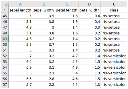
When you are given any data for analysis, in many cases the first thing you have to do preprocess the data in such a form that can be processed by the neural network that you will use. The first step is to remove all the text since those cannot be handled directly by neural network.
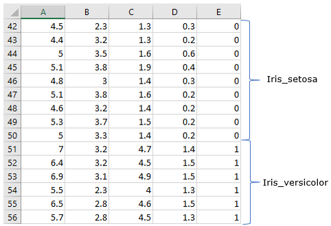
You can just remove the column title test this is not used by the neural network, but the text indicating the class of the iris cannot simply be removed sinec this is critical information for the dataset. So you need to change those text into some form of numbers. What number to be used is completely up to you. In this example, I replaced the text 'Iris-setosa' as 0 and replaced 'iris-versicolor' as 1. You may use '-1' and '1' for these or any other numbers. But in that case, you may need to change some properties of the neural network that you will use. Just give it try to use different numbers and see if the code at the end of this page works as expected. If it is not working as expected, try modifying properties of the network (like activation function) to make it work. All of these trial and error process would be good learning process.
With the data that are made up of all numbers, I did the followings.
iris_data = csvread('iris_dat.csv'); % Read the data file and store them as a matrix.
Then, generate a sequence of random integers ranging between 1 and the size of table(total rows of the table).
rng(1);
shuffled_index = randi([1 length(iris_data)],1,length(iris_data));
Then, rearrange the rows of the data using the random number.
iris_data = iris_data(shuffled_index,:);
Split the dataset into two groups. One for training and the other one for testing.
iris_Train = iris_data(1:50,:); % take out the first 50 rows for training
iris_Test = iris_data(51:150,:); % take out the next 100 rows for testing after the training.
There is another steps of modification. In the dataset, we have 4 columns that can be used for the input of the neural network and one colum (class column) that can be used as output. However, the network that I will use in this example is single perceptron with only two input. So I will take out only two columns (first and third) from the dataset as follows.
pList = [iris_Train(:,1)'; iris_Train(:,3)'];
And then take out the last colum to be used as training output as follows.
tList = iris_Train(:,5)';
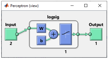
Now a create a network and configure it as single perceptron and initialize the weight and bias as follows.
net = perceptron;
net = configure(net,[0;0],[0]);
net.layers{1}.transferFcn = 'logsig';
net.b{1} = [1];
w = [0.2 0.5];
net.IW{1,1} = w;
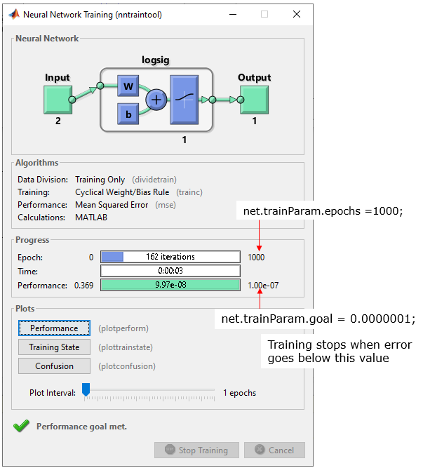
Now set the properties that affects the training process as below. There are many more training parameters and you will see more on those properties in other examples.
net.performFcn = 'mse';
net.trainParam.epochs =1000;
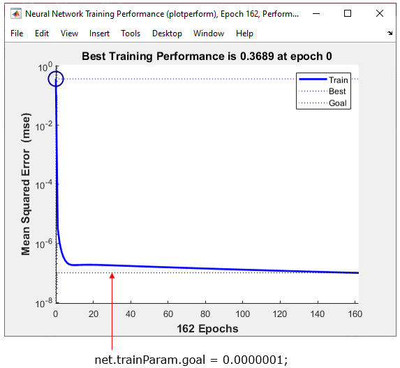
net.trainParam.goal = 0.0000001;
Then train the network and the result is as follows.
net = train(net,pList,tList);
Following is the result of the training. As shown in the graph on the left, you see the two categories are cleared separated by the network (single line).
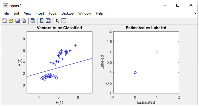
If you are interested in the training procedure, check out the performance as shown below.
|
iris_data = csvread('iris_dat.csv'); rng(1); shuffled_index = randi([1 length(iris_data)],1,length(iris_data));
iris_data = iris_data(shuffled_index,:);
iris_Train = iris_data(1:50,:); iris_Test = iris_data(51:150,:);
pList = [iris_Train(:,1)'; iris_Train(:,3)']; tList = iris_Train(:,5)';
subplot(1,2,1); plotpv(pList,tList);
net = perceptron; net.performFcn = 'mse'; net = configure(net,[0;0],[0]);
net.layers{1}.transferFcn = 'logsig'; net.layers{1}.name = net.layers{1}.transferFcn;
net.b{1} = [1]; w = [0.2 0.5]; net.IW{1,1} = w;
net.trainParam.epochs =1000; net.trainParam.goal = 0.0000001; net = train(net,pList,tList);
plotpc(net.IW{1,1},net.b{1})
pList = [iris_Test(:,1)'; iris_Test(:,3)']; tList = iris_Test(:,5)'; view(net);
subplot(1,2,2); y = net(pList); plot(y,tList,'bo'); axis([-1 2 -1 2]); xlabel('Estimated'); ylabel('Labeled'); title('Estimated vs Labeled'); |
Next Step :