Octave/Matlab Home : www.sharetechnote.com
In this page, I would post a quick reference for Matlab and Octave. (Octave is a GNU program which is designed to provide a free tool that work like Matlab. I don't think it has 100% compatability between Octave and Matlab, but I noticed that most of basic commands are compatible. I would try to list those commands that can work both with Matlab and Octave). All the sample code listed here, I tried with Octave, not with Matlab.
There are huge number of functions which has not been explained here, but I would try to list those functions which are most commonly used in most of matlab sample script you can get. My purpose is to provide you the set of basic commands with examples so that you can at least read the most of sample script you can get from here and there (e.g, internet) without overwhelming you. If you get familiar with these minimal set of functionality, you would get some 'feeling' about the tool and then you would make sense out of the official document from Mathworks or GNU Octave which explains all the functions but not so many examples.
I haven't completed 'what I think is the minimum set' yet and I hope I can complete within a couple of weeks. Stay tuned !!!
Vector (One Dimmensional Array)
- Creating a vector
- Creating a vector with linspace()
- Mathematical Operation
- Applying Functions
- Referencing the elements
- Concatenating Vectors
- Rearranging Elements
- Getting the size of the vector
- Converting a Vector into a Matrix (Converting one dimmensional array into multi dimensional array)
Matrix (Two or Higher Dimmensional Array)
- Creating a Matrix
- Mathematical Operation (Basic Operators)
- Matrix specific operations
- Rearranging Elements
- Single Random Number between 0 and 1
- Single Random Number between a and b
- N Random Number between 0 and 1
- N Random Number between a and b
- Single Random Integer between 0 and N
- Single Random Integer between a and b
- N Random Number between 0 and N
- N Random Number between a and b
- Plot only one data set (y axis data only)
- Plot a set of data ((x,y) sequence)
- x,y Axis Range
- Graph Title, Axis Label
- Graph Format and Color
- Graph with Filled Marker
- AspectRatio
- Multiple Plots in a single graph area using plot
- Multiple Plots in a single graph area using hold on
- Multiple Plots in a single graph area using subplot
Vector (One Dimmensional Array)
Method 1 : v = [ value value value value ...]
Ex)
|
Input |
v = [ 1 2 4 7 2 1] |
|
Output |
v = 1 2 4 7 2 1 |
Method 2 : v = start:step:end
Ex)
|
Input |
v=1:0.2:2 |
|
Output |
v = 1.0000 1.2000 1.4000 1.6000 1.8000 2.0000 |
< Creating a vector with linspace >
Method 1 : v = linspace(start_value,end_value,num_of_data)
Ex)
|
Input |
v = linspace(1,4,10) |
|
Output |
v = 1.0000 1.3333 1.6667 2.0000 2.3333 2.6667 3.0000 3.3333 3.6667 4.0000 |
Case 1 : v = vector1 + vector2
Ex)
|
Input |
v1=[1 2 3 4]; v2=[5 6 7 8]; v=v1 + v2 |
|
Output |
v = 6 8 10 12 |
Case 2 : v = vector1 - vector2
Ex)
|
Input |
v1=[1 2 3 4]; v2=[5 6 7 8]; v=v1 - v2 |
|
Output |
v = -4 -4 -4 -4 |
Case 3 : v = vector1 . vector2 (Inner Product)
Ex)
|
Input |
v1=[1 2 3 4]; v2=[5 6 7 8]; v=v1 * v2' // Note : I put the transpose operator (') here. Try v = v1*v2 and see what happen. |
|
Output |
v = 70 |
Case 4 : v = vector1 x vector2 (multiplication of each elements)
Ex)
|
Input |
v1=[1 2 3 4]; v2=[5 6 7 8]; v=v1 .* v2 // Note : I used .*, not * . Try v = v1*v2 and see what happen. |
|
Output |
v = 5 12 21 32 |
Case 5 : v = vector1 / vector2 (division of each elements)
Ex)
|
Input |
v1=[1 2 3 4]; v2=[5 6 7 8]; v=v1 ./ v2 // Note : I used ./, not / |
|
Output |
v = 0.20000 0.33333 0.42857 0.50000 |
Case 6 : v = scalar + vector2
Ex)
|
Input |
v1 =[1 2 3 4]; s = 2; v= s + v1 // Note : In this case, v = s .+ v1 will give the same result |
|
Output |
v = 3 4 5 6 |
Case 7 : v = scalar x vector2
Ex)
|
Input |
v1 =[1 2 3 4]; s = 2; v= s .* v1 // Note : In this case, v = s * v1 will give the same result |
|
Output |
v = 2 4 6 8 |
Case 1 : v = function(vector)
Ex)
|
Input |
v1 =[1 2 3 4]; v= sin(v1) |
|
Output |
v = 0.84147 0.90930 0.14112 -0.75680 |
Ex)
|
Input |
v1 =[1 2 3 4]; v= v1.^2 + 2 .* v1 + cos(v1) |
|
Output |
v = 3.5403 7.5839 14.0100 23.3464 |
Case 1 : v = vector (index)
Ex)
|
Input |
v1 =[1 2 3 4]; v= v1(3) |
|
Output |
v = 3 |
Case 2 : v = vector ([index range])
Ex)
|
Input |
v1 =[1 2 3 4]; v= v1([1:3]) |
|
Output |
v = 1 2 3 |
Case 3 : v = vector ([index list])
Ex)
|
Input |
v1 =[1 2 3 4]; v= v1([4 2 3]) |
|
Output |
v = 4 2 3 |
Case 4 : v = vector (end)
Ex)
|
Input |
v1 =[1 2 3 4]; v= v1(end) |
|
Output |
v = 4 |
Case 1 : v = [v1 v2] // All the logic is same
Ex)
|
Input |
v1 =[1 2 3 4]; v2 =[5 6 7 8]; v= [v1 v2] |
|
Output |
v = 1 2 3 4 5 6 7 8 |
Ex)
|
Input |
v1 =[1 2 3 4]; v2 =[5 6 7 8]; v= [v1 v2 -v1] |
|
Output |
v = 1 2 3 4 5 6 7 8 -1 -2 -3 -4 |
Ex)
|
Input |
v=[]; // create a variable named 'v' and initialize it with an empty array for i = 1:10 v=[v i]; end v |
|
Output |
v = 1 2 3 4 5 6 7 8 9 10 |
< Rearranging Elements - shift() >
Case 1 : v = shift(vector,N) // Where N is a Positive Number
Ex)
|
Input |
v1 = [1 2 3 4 5 6 7 8 9 10]; v = shift(v1,3) |
|
Output |
v = 8 9 10 1 2 3 4 5 6 7 |
Case 2 : v = shift(vector,N) // Where N is a Negative Number
Ex)
|
Input |
v1 = [1 2 3 4 5 6 7 8 9 10]; v = shift(v1,-3) |
|
Output |
v = 4 5 6 7 8 9 10 1 2 3 |
< Getting the size of a vector : size() >
Case 1 : v = size(v) // returns number of cols and number of rows of v
Ex)
|
Input |
t = 0:0.1:10; size(t) |
|
Output |
ans = 1 101 |
Case 2 : v = size(v,1) // returns the number of rows of v
Ex)
|
Input |
t = 0:0.1:10; size(t,1) |
|
Output |
ans = 1 |
Case 3 : v = size(v,2) // returns the number of rows of v
Ex)
|
Input |
t = 0:0.1:10; size(t,2) |
|
Output |
ans = 101 |
< Getting the size of a vector : length() >
Case 1 : v = length(v) // returns number of elements of v
Ex)
|
Input |
t = 0:0.1:10; length(t) |
|
Output |
ans = 101 |
Case 1 : v = reshape(vector,rows,cols)
Ex)
|
Input |
v1 = [1 2 3 4 5 6 7 8 9 10]; v = reshape(v1,2,5) // Note : Number of matrix elements and Vector elements should be same |
|
Output |
v = 1 2 3 4 5 6 7 8 9 10 |
Matrix (Two or Higher Dimmensional Array)
Method 1 : m = [ value value value ; value value value ; ...]
Ex)
|
Input |
m = [1 2 3; 4 5 6; 7 8 9] |
|
Output |
m = 1 2 3 4 5 6 7 8 9 |
Method 2 : m = [ vector ; vector ; ...]
Ex)
|
Input |
v1 = [1 2 3]; v2 = [4 5 6]; v3 = [7,8,9]; m = [v1; v2; v3] |
|
Output |
m = 1 2 3 4 5 6 7 8 9 |
< Creating an Identity Matrix >
Method 1 : m = eye(M) // M x M identity matrix
Ex)
|
Input |
m = one(3) |
|
Output |
m = 1 0 0 0 1 0 0 0 1 |
< Creating M x N Zero Matrix >
Method 1 : m = zeros(M,N)
Ex)
|
Input |
m = zeros(4,2) |
|
Output |
m = 0 0 0 0 0 0 0 0 |
Method 2 : m = zeros(M) // M x M square matrix
Ex)
|
Input |
m = zeros(3) |
|
Output |
m = 0 0 0 0 0 0 0 0 0 |
< Creating a M x N one matrix >
Method 1 : m = ones(M,N)
Ex)
|
Input |
m = ones(4,2) |
|
Output |
m = 1 1 1 1 1 1 1 1 |
Method 2 : m = ones(M) // M x M square matrix
Ex)
|
Input |
m = one(3) |
|
Output |
m = 1 1 1 1 1 1 1 1 1 |
Case 1 : m = matrix1 + matrix 2;
Ex)
|
Input |
m1 = [1 2 3; 4 5 6; 7 8 9]; m2 = [9 8 7; 6 5 4; 3 2 1]; m = m1 + m2 |
|
Output |
m = 10 10 10 10 10 10 10 10 10 |
Case 2 : m = matrix1 .* matrix 2; // element by element multiplication
Ex)
|
Input |
m1 = [1 2 3; 4 5 6; 7 8 9]; m2 = [9 8 7; 6 5 4; 3 2 1]; m = m1 .* m2 |
|
Output |
m = 9 16 21 24 25 24 21 16 9 |
Case 3 : m = matrix1 * matrix 2; // Inner Product
Ex)
|
Input |
m1 = [1 2 3; 4 5 6; 7 8 9]; m2 = [9 8 7; 6 5 4; 3 2 1]; m = m1 * m2 |
|
Output |
m = 30 24 18 84 69 54 138 114 90 |
Case 4 : m = matrix1 .^ n; // power of n for each element
Ex)
|
Input |
m1 = [1 2 3; 4 5 6; 7 8 9]; m2 = [9 8 7; 6 5 4; 3 2 1]; m = m1 .^ 2; |
|
Output |
m = 1 4 9 16 25 36 49 64 81 |
Case 5 : m = matrix1 ^ n; // matrix power
Ex)
|
Input |
m1 = [1 2 3; 4 5 6; 7 8 9]; m2 = [9 8 7; 6 5 4; 3 2 1]; m = m1 ^ 2; |
|
Output |
m = 30 36 42 66 81 96 102 126 150 |
Case 6 : tm = m'; // transpose matrix
Ex)
|
Input |
m = [1 2 3; 6 5 4; 7 3 9]; tm=m' |
|
Output |
tm = 1 6 7 2 5 3 3 4 9 |
Case 7 : im = inv(m); // take the inverse matrix
Ex)
|
Input |
m = [1 2 3; 6 5 4; 7 3 9]; im=inv(m) |
|
Output |
im = -0.47143 0.12857 0.10000 0.37143 0.17143 -0.20000 0.24286 -0.15714 0.10000 |
Case 8 : im = det(m); // take the determinant of the matrix
Ex)
|
Input |
m = [1 2 3; 6 5 4; 7 3 9]; dm=det(m) |
|
Output |
dm = -70 |
Case 1 : Eigenvalue and Eigenvector
Ex)
|
Input |
A = [1.01 0;0 0.9]; [v,d]=eig(A) |
|
Output |
v =
0 1 1 0
d =
Diagonal Matrix
0.90000 0 0 1.01000 |
|
Input |
A*v |
|
Output |
ans =
0.00000 1.01000 0.90000 0.00000 |
|
Input |
v*d |
|
Output |
ans =
0.00000 1.01000 0.90000 0.00000 |
< Rearranging Elements - circshift() >
Case 1 : m = circshift(m1,N) // Where N is a positive Number. This shift rows
Ex)
|
Input |
m1 = [1 2 3; 4 5 6; 7 8 9]; m = circshift(m1,1) |
|
Output |
m = 7 8 9 1 2 3 4 5 6 |
Case 2 : m = circshift(m1,N) // Where N is a Negative Number. This shift rows
Ex)
|
Input |
m1 = [1 2 3; 4 5 6; 7 8 9]; m = circshift(m1,-1) |
|
Output |
m = 4 5 6 7 8 9 1 2 3 |
Case 3 : m = circshift(m1,[0 N]) // Where N is a Positive Number. This shift cols
Ex)
|
Input |
m1 = [1 2 3; 4 5 6; 7 8 9]; m = circshift(m1,[0 1]) |
|
Output |
m = 3 1 2 6 4 5 9 7 8 |
Case 3 : m = circshift(m1,[0 N]) // Where N is a Negative Number. This shift cols
Ex)
|
Input |
m1 = [1 2 3; 4 5 6; 7 8 9]; m = circshift(m1,[0 1]) |
|
Output |
m = 2 3 1 5 6 4 8 9 7 |
< Rearranging Eelemetns - resize() >
Case 1 : m = resize(m1,M,N,..)
// Resize Matrix m1 to be an M x N x .. matrix, where M, N is smaller than the original matrix
Ex)
|
Input |
m1 = [1 2 3; 4 5 6; 7 8 9]; m = resize(m1,3,2) |
|
Output |
m = 1 2 4 5 7 8 |
Case 2 : m = resize(m1,M,N,..)
// Resize Matrix m1 to be an M x N x .. matrix, where M or N is smaller than the original matrix
Ex)
|
Input |
m1 = [1 2 3; 4 5 6; 7 8 9]; m = resize(m1,3,2) |
|
Output |
m = 1 2 3 0 0 4 5 6 0 0 7 8 9 0 0 0 0 0 0 0 |
Case 3 : m = resize(m1,M) // Resize Matrix m1 to be an M x M matrix
Ex)
|
Input |
m1 = [1 2 3; 4 5 6; 7 8 9]; m = resize(m1,2) |
|
Output |
m = 1 2 4 5 |
< Single Random Number between 0 and 1 >
Case 1 : r = rand(1,1)
Ex)
|
Input |
r = rand(1,1); |
|
Output |
r = 0.36579 |
< Single Random Number between a and b >
Case 1 : r = a + (b-a)*rand(1,1)
Ex)
|
Input |
a = 2; b = 5; r = a + (b-a)*rand(1,1) |
|
Output |
r = 2.36579 |
< N Random Number between 0 and 1 >
Case 1 : r = rand(1,N)
Ex)
|
Input |
r = rand(1,5); |
|
Output |
r = 0.199260 0.814680 0.687995 0.666070 0.013624 |
< N Random Number between a and b >
Case 1 : r = a + (b-a)*rand(1,N)
Ex)
|
Input |
a = 2; b = 5; r = a + (b-a)*rand(1,5) |
|
Output |
r = 2.6419 4.1258 4.7051 2.0323 3.4711 |
< Single Random Integer between 0 and N >
Case 1 : r = randi(N)
Ex)
|
Input |
r = randi(10); |
|
Output |
r = 5 |
< Single Random Integer between a and b >
Case 1 : r = randi([a b]) // where a and b are all integer
Ex)
|
Input |
r = randi([100 200]); |
|
Output |
r = 163 |
< N Random Number between 0 and M >
Case 1 : ri = randi(M,1,N)
Ex)
|
Input |
r = randi(100,1,10); |
|
Output |
r = 20 39 63 81 67 54 34 16 93 19 |
< N Random Number between a and b >
Case 1 : ri = randi([a b],1,N)
Ex)
|
Input |
r = randi([100 200],1,10); |
|
Output |
r = 150 114 142 189 172 103 190 102 196 194 |
2D Graph
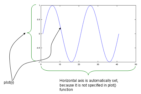
< Plot only one data set (y axis data only) >
Case 1 : plot(y); // specify y (independent variable) only
Ex)
|
Input |
x = -2*pi:1/10*pi:2*pi; y=sin(x); plot(y); |
|
Output |
|
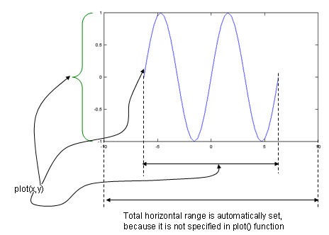
< Plot a set of data ((x,y) sequence) >
Ex)
|
Input |
x = -2*pi:1/10*pi:2*pi; y=sin(x); plot(x,y); |
|
Output |
|
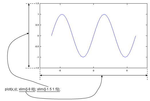
Case 1 : xlim([xmin xmax]); ylim([ymin ymax]);
Ex)
|
Input |
x = -2*pi:1/10*pi:2*pi; y=sin(x); plot(x,y); xlim([-8 8]); ylim([-1.5 1.5]); |
|
Output |
|
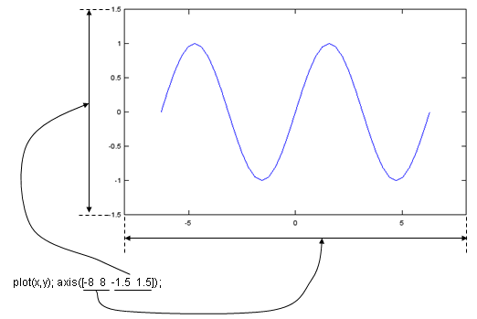
Case 2 : axis([xmin xmax ymin ymax]);
Ex)
|
Input |
x = -2*pi:1/10*pi:2*pi; y=sin(x); plot(x,y); axis([-8 8 -1.5 1.5]); |
|
Output |
|
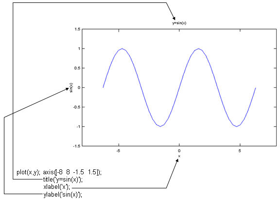
Case 1 : title('text');
xlabel('text');
ylabel('text');
Ex)
|
Input |
x = -2*pi:1/10*pi:2*pi; y=sin(x); plot(x,y); xlim([-8 8]); ylim([-1.5 1.5]);title('y=sin(x)'); xlabel('x');ylabel('sin(x)'); |
|
Output |
|
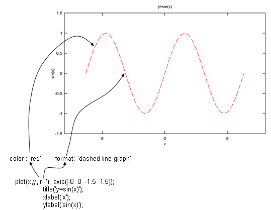
Case 1 : plot(x,y,'format');
`-' : solid line.
`.' : dotted line.
`--' : dashed line
`^' : triangular mark
`+' : + mark
`*' : * mark
`o' : o (circle) mark
`x' : x mark
Ex)
|
Input |
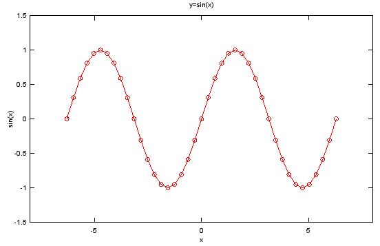
x = -2*pi:1/10*pi:2*pi; y=sin(x); plot(x,y,'r--'); xlim([-8 8]); ylim([-1.5 1.5]);title('y=sin(x)'); xlabel('x');ylabel('sin(x)'); |
|
Output |
|
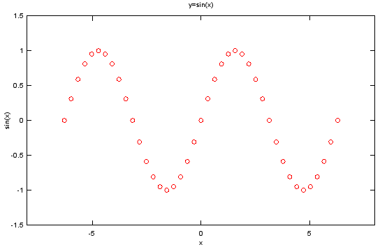
Ex)
|
Input |
x = -2*pi:1/10*pi:2*pi; y=sin(x); plot(x,y,'ro'); xlim([-8 8]); ylim([-1.5 1.5]);title('y=sin(x)'); xlabel('x');ylabel('sin(x)'); |
|
Output |
|
Ex)
|
Input |
x = -2*pi:1/10*pi:2*pi; y=sin(x); plot(x,y,'ro-'); xlim([-8 8]); ylim([-1.5 1.5]);title('y=sin(x)'); xlabel('x');ylabel('sin(x)'); |
|
Output |
|
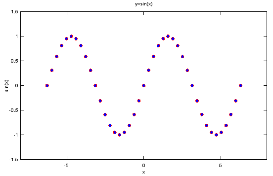
Case 1 : MarkerFaceColor,[r g b] // r,g,b value is range between 0 and 1.
Ex)
|
Input |
x = -2*pi:1/10*pi:2*pi; y=sin(x); plot(x,y,'ro','MarkerFaceColor',[0 0 1]); axis([-8 8 -1.5 1.5]); title('y=sin(x)'); xlabel('x');ylabel('sin(x>< 0 1]); |
|
Output |
|
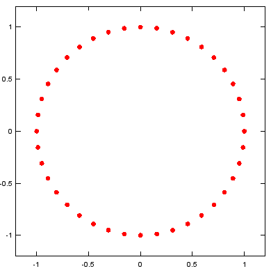
Case 1 : daspect([xratio yratio])
Ex)
|
Input |
t=0:2*pi/40:2*pi; e1 = exp(t*j); plot(real(e1),imag(e1),'ro','MarkerFaceColor',[1 0 0]); axis([-1.2 1.2 -1.2 1.2]);daspect([1 1]); |
|
Output |
|
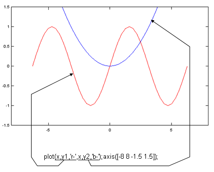
< Multiple Plots in a single graph area using plot >
Case 1 : plot(x1,y1,'format1',x2,y2,'format2',...)
Ex)
|
Input |
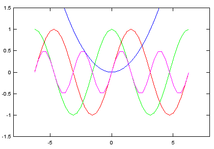
x = -2*pi:1/10*pi:2*pi; y1=sin(x); y2=0.1 .* x .^2; plot(x,y1,'r-',x,y2,'b-');axis([-8 8 -1.5 1.5]); |
|
Output |
|
< Multiple Plots in a single graph area using hold on >
Ex)
|
Input |
x = -2*pi:1/10*pi:2*pi; y1=sin(x); y2=cos(x); y3=0.1.*x.^2; y4=sin(x).*cos(x); subplot(2,2,1); plot(x,y1,'r-');axis([-8 8 -1.5 1.5]);hold on; subplot(2,2,2); plot(x,y2,'g-');axis([-8 8 -1.5 1.5]);hold on; subplot(2,2,3); plot(x,y3,'b-');axis([-8 8 -1.5 1.5]);hold on; subplot(2,2,4); plot(x,y4,'m-');axis([-8 8 -1.5 1.5]); |
|
Output |
|
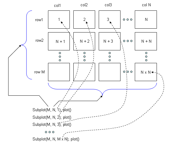
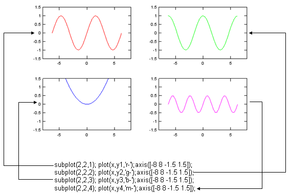
< Multiple Plots in a single graph area using subplot >
Case 1 : Subplot(M, N, 1); plot()
Subplot(M, N, 2); plot()
Subplot(M, N, 3); plot()
...
Subplot(M, N, M x N); plot()
Ex)
|
Input |
x = -2*pi:1/10*pi:2*pi; y1=sin(x); y2=cos(x); y3=0.1.*x.^2; y4=sin(x).*cos(x); subplot(2,2,1); plot(x,y1,'r-');axis([-8 8 -1.5 1.5]); subplot(2,2,2); plot(x,y2,'g-');axis([-8 8 -1.5 1.5]); subplot(2,2,3); plot(x,y3,'b-');axis([-8 8 -1.5 1.5]); subplot(2,2,4); plot(x,y4,'m-');axis([-8 8 -1.5 1.5]); |
|
Output |
|
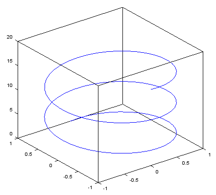
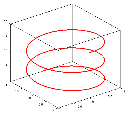
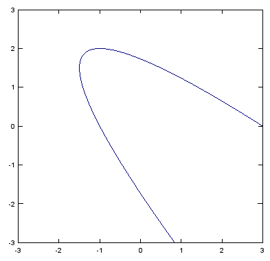
< plot3 - 3D Parametric Plot >
Ex)
|
Input |
t = linspace(0,5*pi,100); plot3(sin(t),cos(t),t) |
|
Output |
|
< plot3 - 3D Parametric Plot - linewidth, color>
Ex)
|
Input |
t = linspace(0,5*pi,100); plot3(sin(t),cos(t),t,'linewidth',3,'color','r'); |
|
Output |
|
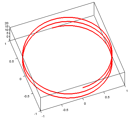
< plot3 - 3D Parametric Plot - view >
view(angle_around_z_axis, angle_around_y_axis) // angle in degree
Ex)
|
Input |
t = linspace(0,5*pi,100); plot3(sin(t),cos(t),t,'linewidth',3,'color','r'); view(-20,80); |
|
Output |
|
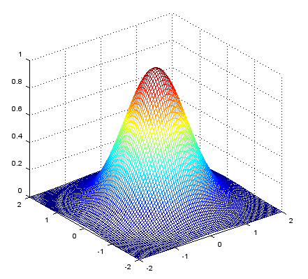
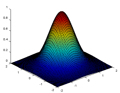
Ex)
|
Input |
xstep = -2:.05:2; ystep = -2:.05:2; [X,Y] = meshgrid(xstep,ystep); Z = exp(-(X.^2+Y.^2)); mesh(X,Y,Z); |
|
Output |
|
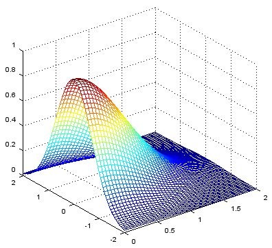
axis([xmin xmax ymin ymax zmin zmax])
Ex)
|
Input |
xstep = -2:.05:2; ystep = -2:.05:2; [X,Y] = meshgrid(xstep,ystep); Z = exp(-(X.^2+Y.^2)); mesh(X,Y,Z); axis([0 2 -2 2 0 1]); |
|
Output |
|
Ex)
|
Input |
xstep = -2:.05:2; ystep = -2:.05:2; [X,Y] = meshgrid(xstep,ystep); Z = exp(-(X.^2+Y.^2)); surface(X,Y,Z); view(-40,30); |
|
Output |
|
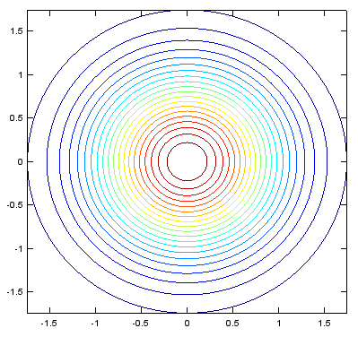
Ex)
|
Input |
xstep = -2:.05:2; ystep = -2:.05:2; [X,Y] = meshgrid(xstep,ystep); Z = exp(-(X.^2+Y.^2)); contour(X,Y,Z,20); |
|
Output |
|
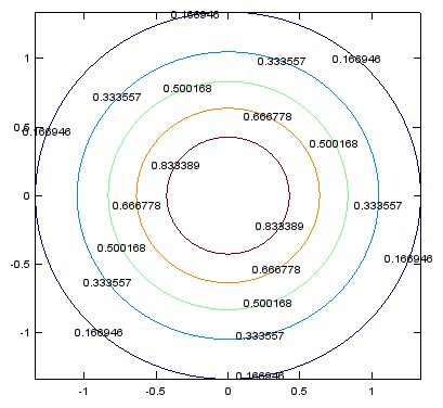
< contour - Labeling the level >
Ex)
|
Input |
xstep = -2:.05:2; ystep = -2:.05:2; [X,Y] = meshgrid(xstep,ystep); Z = exp(-(X.^2+Y.^2)); [c,h]=contour(X,Y,Z,5); clabel(c,h); |
|
Output |
|
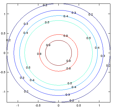
< contour - forcing contour lines >
Ex)
|
Input |
xstep = -2:.05:2; ystep = -2:.05:2; [X,Y] = meshgrid(xstep,ystep); Z = exp(-(X.^2+Y.^2)); [c,h]=contour(X,Y,Z,[0.0 0.2 0.3 0.4 0.5 0.8 0.9]); clabel(c,h); |
|
Output |
|
Ex)
|
Input |
xstep = -3:.05:3; ystep = -3:.05:3; [X,Y] = meshgrid(xstep,ystep); Z=X.^2 .+ 2.*X.*Y .+ Y.^2 - 2.*X; contour(X,Y,Z,[3,3]); % implicit plot for X.^2 .+ 2.*X.*Y .+ Y.^2 - 2.*X = 3 |
|
Output |
|
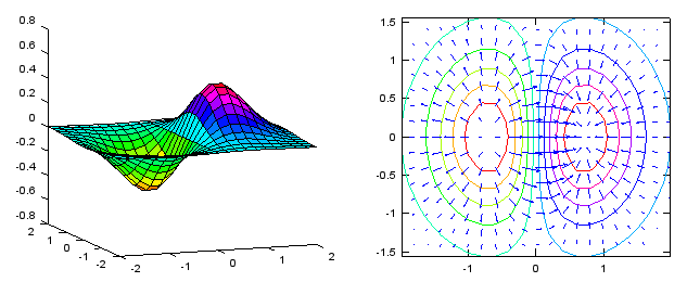
< Vector Plot - Gradient Plot >
Ex)
|
Input |
[X,Y] = meshgrid(-2:.2:2); Z = X.*exp(-X.^2 - Y.^2); [DX,DY] = gradient(Z,.2,.2);
subplot(1,2,1); surface(X,Y,Z); view(-20,10);
subplot(1,2,2); contour(X,Y,Z); hold on quiver(X,Y,DX,DY); colormap hsv hold off |
|
Output |
|
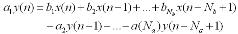
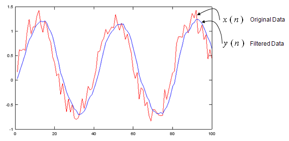
Apply the Digital Filter described as below. As you see in the mathematical description, you can apply both FIR and IIR applying the tab values.
Ex)
|
Input |
a = 1; b = [0.2 0.2 0.2 0.2 0.2]; t = linspace(0,5*pi,100); x = sin(t) .+ 0.5*rand(1,100);
y = filter(b,a,x); plot(x,'r-',y,'b-'); |
|
Output |
|
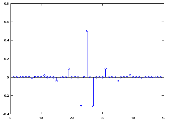
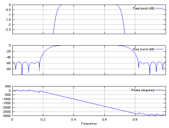
Case 1 : b = fir1(N,[pass_L,pass_R])
// Generate N tap Bandpass Filter with passband [pass_L,pass_R]. 0 < pass_L,pass_R < 1
Ex)
|
Input |
b = fir1(48,[0.25 0.75]); stem(b); figure; freqz(b,1,512); |
|
Output |
|
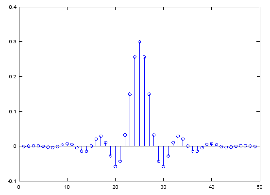
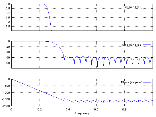
Case 2 : b = fir1(N,pass_R,'low')
// Generate N tap Lowpass Filter with passband [0,pass_R]. 0 < pass_R < 1
Ex)
|
Input |
b = fir1(48,0.3,'low'); stem(b); figure; freqz(b,1,512); |
|
Output |
|
Case 3 : b = fir1(N,pass_L,'high')
// Generate N tap Highpass Filter with passband pass_L. 0 < pass_L < 1
Ex)
|
Input |
b = fir1(48,0.7,'high'); stem(b); figure; freqz(b,1,512); |
|
Output |
|
Case 4 : b = fir1(N,[stop_L stop_R],'stop')
// Generate N tap Bandstop Filter with bandstop between stop_L and stop_R. 0 < stop_L, stop_R < 1
Ex)
|
Input |
b = fir1(48,[0.45 0.55],'stop'); stem(b); figure; freqz(b,1,512); |
|
Output |
|
Case 1 : b = fir2(N,[f1,f2,f3,...,fm],[mag1,mag2,mag3,...,magM])
// Generate N tap Filter with aribitrary passband definition specified by [f1,f2,f3,...,fm],[mag1,mag2,mag3,...,magM]
Ex)
|
Input |
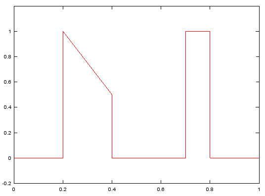
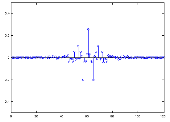
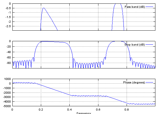
f=[0, 0.2, 0.2, 0.4, 0.4, 0.7, 0.7, 0.8, 0.8, 1]; m=[0, 0, 1, 1/2, 0, 0, 1, 1, 0, 0]; b=fir2(120,f,m);
figure; plot(f,m,'r-');axis([0 1 -0.2 1.2]); figure; stem(b);axis([0,length(b),-0.5,0.5]); figure; freqz(b,1,512); |
|
Output |
|
Case 1 : freqz(b,a,NoOfFrequencyPoints)
// Produce frequency response plot (magnitude and phase vs frequency) with IIR filter coefficient vector b and a. (In case of FIR filter, set a to be 1).
Ex)
|
Input |
b = fir1(48,[0.25 0.75]); freqz(b,1,512); |
|
Output |
|
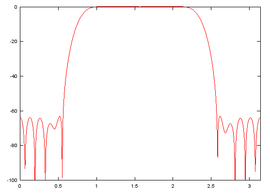
Case 2 : [h,w] = freqz(b,a,NoOfFrequencyPoints)
// return the numerical data of frequency response with IIR filter coefficient vector b and a. (In case of FIR filter, set a to be 1). h returns the magnitude values and w returns frequency point values.
Ex)
|
Input |
b = fir1(48,[0.25 0.75]); [h,w]=freqz(b,1,512); plot(w,10 .* log(abs(h)),'r-');axis([0 pi,-100,0]); |
|
Output |
|