|
Matlab/Octave |
||
|
Filter Design Tutorial
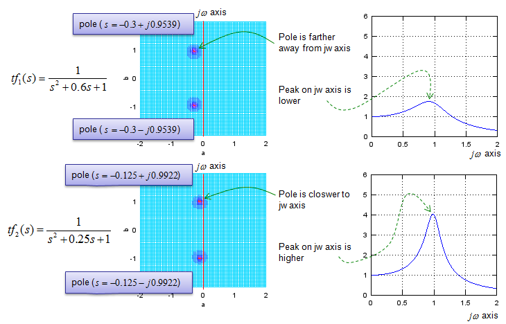
Example 1 :
w = 0:0.01:2; s = j * w; Tf = 1 ./ (s.^2 + 0.6 .* s .+ 1); Tf_abs = abs(Tf); plot(w,Tf_abs);grid();
Example 2 :
re = -2:.05:2; im = -2:.05:2;
[a,b] = meshgrid(re,im); s = (a + b*j);
Tf = 1 ./ (s.^2 + 0.6 .* s .+ 1); Tf_abs = abs(Tf);
mesh(X,Y,Tf_abs);xlabel('a');ylabel('b');zlabel('|Tf(s)|');
re = -2:.05:2; im = -2:.05:2;
[a,b] = meshgrid(re,im); s = (a + b*j);
Tf = 1 ./ (s.^2 + 0.6 .* s .+ 1); Tf_abs = abs(Tf);
mesh(X,Y,Tf_abs); xlabel('a');ylabel('b');zlabel('|Tf(s)|'); view(0,90); zmax = 20; zmin = -10; caxis([-zmax zmax]); colormap(hsv(20));
re = -2:.025:2; im = -2:.025:2;
[a,b] = meshgrid(re,im); s = (a + b*j);
Tf = 1 ./ (s.^2 + 0.6 .* s .+ 1); Tf_abs = abs(Tf);
contour(a,b,Tf_abs,200); xlabel('a');ylabel('b'); xlim([-2 2]);ylim([-2 2]);zlim([0 10]);
Example 3 :
download matlab/octable .m file
re = -3:.05:3; im = -3:.05:3; a = 0.4; b = 1.0; z_List = [ 0 + 1.2*j 0 + 1.8*j 0 - 1.2*j, 0 - 1.8*j]; p_List = [ a*cos(pi/2+pi/12)+b*sin(pi/2+pi/12)*j a*cos(pi/2+4*pi/12)+b*sin(pi/2+4*pi/12)*j a*cos(pi/2+pi/12)-b*sin(pi/2+pi/12)*j a*cos(pi/2+4*pi/12)-b*sin(pi/2+4*pi/12)*j];
[X,Y] = meshgrid(re,im); s = (X + Y*j); s_jw = (0 + Y*j);
num = ones(length(X),length(Y));
for i=1:length(z_List) num = num .* (s .- z_List(i)); end;
den = ones(length(X),length(Y));
for i=1:length(z_List) den = den .* (s .- p_List(i)); end;
Zw_num = ones(length(X),length(Y));
for i=1:length(z_List) Zw_num = Zw_num .* (s_jw .- z_List(i)); end;
Zw_den = ones(length(X),length(Y));
for i=1:length(z_List) Zw_den = Zw_den .* (s_jw .- p_List(i)); end;
Zabs = abs(num ./ den ); Zabs = 10 * log10(Zabs); Zarg = arg(num ./ den); Zw = abs(Zw_num ./ Zw_den); Zw = 10 * log10(Zw); Zwarg = arg(Zw_num ./ Zw_den);
zmax = 20; zmin = -10; subplot(2,2,1); mesh(X,Y,Zabs);axis([re(1) re(end) im(1) im(end) zmin zmax]); hold on; plot3(X.*0,Y,Zw, 'linewidth',3,'color','r'); hold off; view(50,10); caxis([-zmax zmax]); colormap(hsv(20)); subplot(2,2,2); mesh(X,Y,Zabs);axis([0 re(end) im(1) im(end) zmin zmax]); hold on; plot3(X.*0,Y,Zw, 'linewidth',3,'color','r'); hold off; view(-90,10); caxis([-zmax zmax]); colormap(hsv(20)); subplot(2,2,3); mesh(X,Y,Zabs);axis([re(1) re(end) im(1) im(end) zmin zmax]); hold on; plot3(X.*0,Y,Zw, 'linewidth',3,'color','r'); hold off; view(0,90); caxis([-zmax zmax]); colormap(hsv(20)); subplot(2,2,4); mesh(X,Y,Zarg);axis([0 re(end) im(1) im(end) -pi pi]); hold on; plot3(X.*0,Y,Zwarg, 'linewidth',3,'color','r'); hold off; view(-90,10);
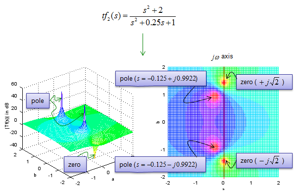
Impact of the location of pole from jw axis
re = -2:.05:2; im = -2:.05:2;
[a,b] = meshgrid(re,im); s = (a + b*j);
Tf = (s.^2 .+ 2) ./ (s.^2 + 0.6 .* s .+ 1); %Tf = 1 ./ (s.^2 + 0.6 .* s .+ 1); Tf_abs = abs(Tf); Tf_abs_log = 10 .* log(Tf_abs);
subplot(1,2,1); mesh(X,Y,Tf_abs_log);xlabel('a');ylabel('b');zlabel('|Tf(s)| in dB');
subplot(1,2,2); mesh(X,Y,Tf_abs_log);xlabel('a');ylabel('b');zlabel('|Tf(s)| in dB'); view(0,90); zmax = 20; zmin = -10; caxis([-zmax zmax]); colormap(hsv(20));
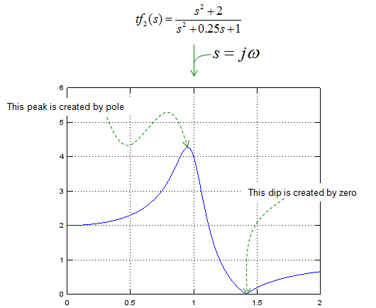
w = 0:0.01:2; s = j * w; Tf = (s.^2 .+ 2) ./ (s.^2 + 0.25 .* s .+ 1); %Tf = 1 ./ (s.^2 + 0.6 .* s .+ 1); Tf_abs = abs(Tf); plot(w,Tf_abs); ylim([0 6]); grid();
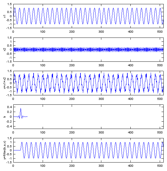
Fs=8e3; Ts=1/Fs; Ns=512; t=[0:Ts:Ts*(Ns-1)]; f1=500; f2=3200; x1=sin(2*pi*f1*t); x2=0.3*sin(2*pi*f2*t); x=x1+x2; a = 1; b = fir1(48,0.35,'low'); y=filter(b,a,x); subplot(5,1,1); plot(x1);ylabel('x1');axis([0,length(x),-1.5,1.5]); subplot(5,1,2); plot(x2);ylabel('x2');axis([0,length(x),-1.5,1.5]); subplot(5,1,3); plot(x);ylabel('x=x1+x2');axis([0,length(x),-1.5,1.5]); subplot(5,1,4); plot(b);ylabel('b');axis([0,length(x),-0.5,0.5]); subplot(5,1,5); plot(y);ylabel('y=filter(b,a,x)');axis([0,length(x),-1.5,1.5]);
|
||