One of the big questions (research area) in adopting Massive MIMO is what kind of reciever model (algorithm) would be the best fit for this technology. As we see in most case, the first idea tend to come from existing technologies and the most common candidates are MRC(Maximum Ratio Combining), ZF (Zero Forcing) and MMSE (Minimum Mean Square Error). You can have general introduction of these reciever technology in ZF and MMSE page. Those pages are only for general introduction, not specifically for Massive MIMO, but you may have some big picture from those pages if you are new to this area.

Before comparing them it helps to say what the receiver is being asked to do. The array collects L observations, one per antenna. Several data streams are mixed into every one of those observations, and the receiver has to recover each stream separately.

Only two things stand in the way. One is thermal noise, which more transmit power reduces. The other is the other streams, which more transmit power does not reduce, because it raises them equally. The three algorithms differ mostly in which of those two they take seriously.

• The efficiency of Massive MIMO Reciever Model
• How to read these performance graphs
• Why the MRC curves flatten and the MMSE curves do not
• MRC, ZF and MMSE : what each one optimizes
• What the two layer structure is, and why 2 x 16
• What the matrix inverse really costs
• So which one would you choose ?
• Reference

The efficiency of Massive MIMO Reciever Model 

Now let's think of what would be the best candidate  for Massive MIMO technology. Of course, there would be no clear answer to this question. The answer might be different depending on how you define the world 'the best' candidate.

I think a single graph from  Nutaq whitepaper titled "Two-Layer Linear Processing for Massive MIMO on the Titan MIMO Platform" (See Reference [1]) would give you a lot of information or idea when you try to chose reciever algorithm. The graph looks as follows.

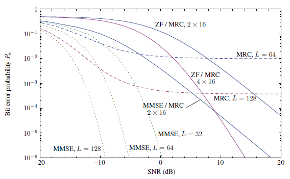
Whenever you are given this kind of graph, it would not make much sense to to you (or would not give you much idea) unless you take very close look. (If you are new to this area, the meaning of graph itself would not be clear .. I will post another introductary page to interpret this kind of performance graph later).

Now let's look more deeply into the graph and see what this graph really try to tell.

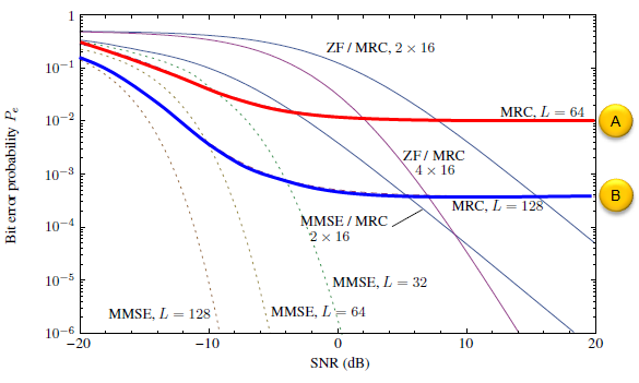
First, let take a look at only two curve (marked in red(A) and blue(B) in the following graph). (A) use 64 antenna and (B) use 128 antenna, and both (A) and (B) use the same algorithm(MRC). You see (B) shows better performance. This is understandable. But you see you would not achieve good enough performance regardless of how many antenna you use. Even with 128 antenna, the performance (error rate) does not improve any further from SNR of roughly 6 dB.

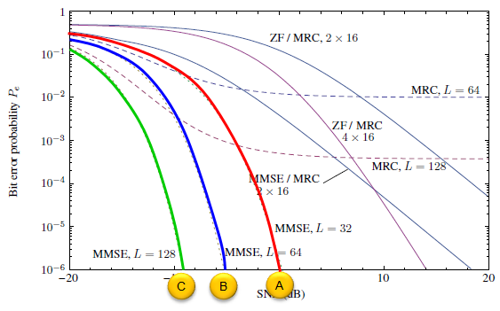
Now, let take a look at following three curves (marked in red(A), blue(B) and green(C) in the following graph). (A) use 32 antenna, (B) use 64 antenna and (C) uses 128. (A),(B) and (C) use the same algorithm (MMSE). You see (B) shows better performance than (A) and (C) performs better than (B). This is understandable. also it seems that these are good enough to use in real life.

It is true if you only think of performance. However, if you look into the MMSE algorithm in MMSE Introduction page, you would notice that this algorithm requires a lot of matrix calculation especially 'matrix inverse' operation. This matrix operation would take exponentially larger processing power (memory, calculation time etc) as the size of the matrix grow larger. So it might become a little bit difficult (or inefficient in terms of processing power and complexity of implementation).

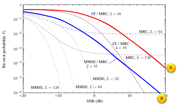
Now, let take a look at another set of curves (marked in red(A) and blue(B) in the following graph). Both (A) and (B) uses the same number of Antenna (32 antenna) but they use different algorithms. One thing you should notice is that these are not using single algorithm for each case, they are using a combined algorithm. In (A), it uses a combined algorithm of ZF and MRC and in (B), it uses a combined algorithm of MMSE and MRC. (I will post another separate page to show the details of how these two algorithm are combined). Here, you only have to see MMSE+MRC (B) shows better performance than ZF+MRC (A).

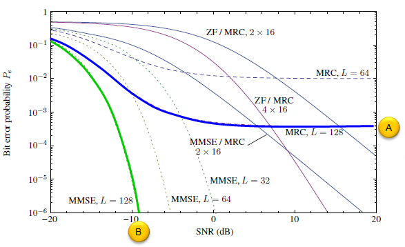
Now let's compare following two curves. As you see, These two cases are using the same number of antenna (128) but using different reciever algorithm( (A) = MRC, (B) = MMSE). You would see that the curve (B) shows much better performance.

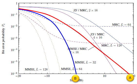
Now let's compare another set of curves. As you see, These two cases are using the same number of antenna (32) but using different reciever algorithm( (A) = MRC+MMSE, (B) = MMSE). You would see that the curve (B) shows much better performance. Which algorithm would you pick for your system ? If you think only of performance itself, you would pick (B), but if you consider the required processing power and complexity, (A) can be a choice as well (This is what Nutaq suggests in the whitepaper. Of course, the final decision is all yours :)

How to read these performance graphs

The page above promises a separate introduction on reading this kind of graph. This section is a short version, enough to follow the curves on this page.

The horizontal axis is SNR in decibels, so moving right means spending more transmit power. The vertical axis is the bit error probability on a log scale, where each gridline is a factor of ten. Better performance is down and to the left.

Two features carry most of the meaning. A steep curve means a small increase in power buys a large drop in errors. A flat curve means extra power buys nothing at all, and that is the more interesting case.

Horizontal distance is the useful measure when comparing two curves. If one curve reaches the same error rate 3 dB to the left of another, it needs half the transmit power. Twenty decibels to the left means one hundredth of the power.

The legend needs decoding too, because it uses two different notations. A label with L gives a plain single layer receiver over that many antennas. A label like 2 x 16 describes the two layer arrangement, and the antenna total is the product.

That table makes the fair comparisons visible. MMSE at L = 32 and MMSE / MRC at 2 x 16 both use 32 antennas. Putting them side by side compares algorithms and not hardware. The same holds for MMSE at L = 64 against ZF / MRC at 4 x 16.

Why the MRC curves flatten and the MMSE curves do not

The observation above is that MRC stops improving beyond about 6 dB, whatever the antenna count. That flattening has a name and a cause, and it is the single most useful thing in the whole graph.

MRC aligns the array towards one stream and adds the antenna outputs in phase. That maximises the wanted signal, and it treats every other stream as though it were noise. Nothing in the algorithm attempts to cancel them.

So raising the transmit power raises the wanted stream and the interfering streams together. Their ratio does not move, and neither does the error rate. The curve goes flat, and the receiver is described as interference limited rather than noise limited.

< Figure 1. Noise limited and interference limited behaviour >

Figure 1 shows the two shapes side by side. The left part of both curves is noise limited, where power still helps. The MRC curve then reaches its floor and stops, while the MMSE curve keeps falling.

More antennas do lower the floor. MRC at L = 64 settles near 1e-2, and MRC at L = 128 settles near 4e-4. Doubling the array moved the floor by more than an order of magnitude, which is a real gain. The floor still exists, and no amount of power reaches past it.

MMSE keeps falling because it uses the structure of the interference instead of ignoring it. Inverting the correlation matrix places nulls towards the interfering streams. What is left is mostly noise, and noise does respond to power.

• A floor means interference, not noise : Extra power lifts wanted and unwanted signals equally, so the ratio is unchanged.
• Antennas lower the floor but never remove it : MRC at 128 antennas is far better than at 64, and still flat.
• Only a receiver that models interference escapes it : That is what the matrix inverse in ZF and MMSE is buying.

MRC, ZF and MMSE : what each one optimizes

The three names appear in the opening paragraph as candidates. Each is best understood by what it tries to make as good as possible. That single choice explains every difference on the graph.

ZF and MMSE both invert a matrix, so they cost about the same. The difference is what they invert. ZF cancels interference whatever it does to the noise, and at low SNR that amplification is severe.

MMSE includes the noise term, so it declines to cancel interference when doing so would cost more in noise than it gains. At high SNR the noise term becomes negligible and the two receivers converge.

That is visible on the graph. The ZF / MRC curves sit well above the MMSE / MRC curves on the left hand side, where noise dominates. The gap narrows towards the right, exactly as the theory says it should.

What the two layer structure is, and why 2 x 16

The page above notes that the combined cases use two algorithms together, and leaves the detail to a later page. The whitepaper title gives the shape of it. Two-Layer Linear Processing means one receiver applied inside groups, and a second applied across them.

The array is divided into equal groups. Each group runs its own small ZF or MMSE receiver, which is the first layer. The group outputs are then combined with MRC, which is the second layer and needs no matrix inverse at all.

< Figure 2. The two layer arrangement behind the 2 x 16 notation >

Figure 2 draws the 2 x 16 case. Two groups of sixteen antennas give 32 antennas in total, and the expensive step is an inverse of size 16 rather than size 32.

The saving follows a simple rule. Inverting an n by n matrix costs about n cubed, so one group of size L costs L cubed. Splitting into G groups of size L over G costs G times that smaller cube, and the ratio between them is G squared.

Two groups therefore save a factor of four. Eight groups save a factor of sixty four. The arrangement becomes more attractive as the array grows, because the number of groups grows with it.

The cost is performance, and on this graph it is large. MMSE at L = 32 reaches an error of 1e-6 at roughly -2 dB. MMSE / MRC at 2 x 16 needs roughly +18 dB for the same point, with the same 32 antennas.

So the two layer version gives up about 20 dB to save a factor of four in the inverse. At two groups that is a poor bargain. The arrangement earns its place on larger arrays, where the saving grows as the square while the loss does not.

What the matrix inverse really costs

One correction is worth making to the paragraph above. Inverting an n by n matrix costs on the order of n cubed operations. That is polynomial growth, not exponential growth, and the difference changes the conclusion.

Exponential growth would rule the method out completely. Cubic growth only makes it expensive, which is why MMSE remains a serious candidate at 128 antennas rather than a theoretical curiosity.

The concrete numbers are easy to carry. Going from a 32 by 32 inverse to a 128 by 128 inverse is four times the size and about sixty four times the work. Going to 8 groups of 16 brings that back down by the same factor of sixty four.

Two further costs are easy to miss. The inverse has to be recomputed whenever the channel changes, so the real figure is operations per second and not operations per symbol. And the matrix has to be estimated first, which costs reference signals rather than arithmetic.

• Cubic, not exponential : Doubling the matrix size multiplies the work by about eight.
• Grouping saves the square of the group count : This is the whole argument for two layer processing.
• The inverse is repeated, not computed once : Channel coherence time decides how often, and that sets the real load.

So which one would you choose ?

The page ends by leaving the decision to the reader, which is the right answer. The choice is easier once the question is split into the two cases that actually occur.

If the system is noise limited, meaning few users and plenty of spatial room, MRC is hard to argue against. It is cheap, it parallelises across antennas, and there is little interference for a smarter receiver to remove.

If the system is interference limited, MRC has a floor and no budget will move it. Then the matrix inverse is not optional, and the only remaining question is whether to pay for it in one piece or in groups.

Massive MIMO makes the first case more common than it used to be. When antennas greatly outnumber users, the channel vectors become close to orthogonal, and the interference that creates the floor becomes small on its own.

That is the deeper reason the topic matters. A large array is partly a way of buying back the receiver complexity that a smaller array would have to spend.

Reference

[1] Two-Layer Linear Processing for Massive MIMO on the TitanMIMO Platform

Sébastien Roy

Dept. of Electrical and Computer Engineering

Université de Sherbrooke

e-mail: s.roy17@usherbrooke.ca

[2] 5G NOW. D3.1 5G Waveform Candidate Selection

[3] Massive MIMO and Small Cells : Improving Energy Efficiency by Optimal Soft-Cell Coordination

Emil Bjornson, Marios Kountouris and Merouane Debbah

Alcatel-Lucent Chair on Flexible Radio, SUPELEC, Gif-sur-Yvette, France

Department of Telecommunications, SUPELEC, Gif-sur-Yvette, France

ACCESS Linnaeus Center, Signal Processing Lab, KTH Royal Institue of Technology, Stockholm, Sweden

[4] Massive MIMO Info Point

[5] Massive MIMO for Next Generation Wireless Systems

Erik G. Larson, ISY, Linkoping University, Sweden

Ove Edfors, Lund University, Sweden

Fredrik Tufvesson, Lund University, Sweden

Thomas L. Marzetta, Bell Labs, Alcatel-Lucent, USA

[6] Scaling up MIMO : Opportunities and Challenges with Very Large Arrays

Fredrik Rusek, Dept. of Electrical and Information Technology, Lund University, Lund, Sweden

Daniel Persson, Dept. of Electrical Engineering (ISY), Linkoping University, Sweden

Buon Kiong Lau, Dept. of Electrical and Information Technology, Lund University, Lund, Sweden

Erik G. Larsson, Dept. of Electrical Engineering (ISY), Linkoping University, Sweden

Thomas L. Marzetta, Bell Laboratories, Alcatel-Lucent, Murray Hill, NJ

Ove Edfors, Dept. of Electrical and Information Technology, Lund University, Lund, Sweden

Fredrik Tufvesson, Dept. of Electrical and Information Technology, Lund University, Lund, Sweden