Propagation Modeling/Channel Impulse Response

The purpose of this page is to describe about how the property of the milimeter wave signal varies as it propagate through the physical media (i.e channel, e.g, air, buldings, trees etc). The modeling of a signal going through a channel is called CIR (Channel Impulse Response) and it is the most fundamental investigation of any wireless communication techologies (If you are not familiar with the term 'Impulse response', refer to Impulse respone page). From this research and investigation, we will eventually obtain more model like Fading Channel Model and MIMO channel model.

This page is mainly motivated by the recent announcement from NYU who decided to share tons of their work for many years and real measurement data, mathematical model as an opensource in Mar 2016 (Refer to Open Source Downloadable 5G Channel Simulator software). This is extremly greatful and thankful, and will definitely invaluable contribution to the whole industry. I think many of you have already seen many presentation slides and papers from this team, and with the opensource you will get the chance to understand those slides/papers as you did all those test by yourself. Reading some of the papers written by the team, I could sense that they have really willingness to share what they have done and trying to help others. Even from very short and very formal papers published in popular journal, you would see they desribe things in very practical way. I strongly recommend you to look into this and search various documents from the team (I put some of them at the reference section).

I will take those material/papers from NYU as a skeleton of this page and keep extending as I learn more from various other sources.

Factors for Channel Impulse Model.
Path Loss Modeling
Delay Spread
Angle of Arrival
How this maps to the 3GPP channel model
Reference
YouTube

Factors for Channel Impulse Model.

A channel model predicts nothing about a property it does not track, so the first question is which properties matter. The three below were not chosen for convenience. Each one limits a different part of the receiver design, and a model that leaves any of them out cannot predict what that part of the receiver will do.

What are the factors defining the nature of the radio channel ? There are many factors, but if I pick only a few important factors, I would list as follows.

i) Path Loss between the transmitter and reciever. This defines how much energy gets lost while the signal is going through the channel (media)

ii) Delay Spread. This indicates how much the signal get dispersed in time domain (in terms of reception timing at Rx Antenna). Refer to Delay Spread page for the detailed concept.

iii) Angle of Arrival. This indicates how the nature of the received signal (mostly the received power and phase) changes with angle of reciever antenna with a specific reference point.

You may add more items to the list, but I think these three would be the most dominant factors defining the channel impulse model. These three factors can be combined into one frame as illustrated below, and I will describe more details on each of the factors.

The drawing puts all three factors on one set of axes. The red curve falling from left to right is received power against distance, which is the path loss view. The blue stems standing on that curve are the arrivals recorded at four successive distances, and their width along the time axis is the delay spread. The green triangle at each point is the receiver antenna, and the elevation and azimuth arrows around it are the two axes an angle of arrival measurement sweeps. Three insets show what each factor becomes once it is plotted on its own. They are a Manhattan path loss scatter at the bottom left, a power delay profile at the top right, and a polar plot of received power against azimuth at the bottom right.

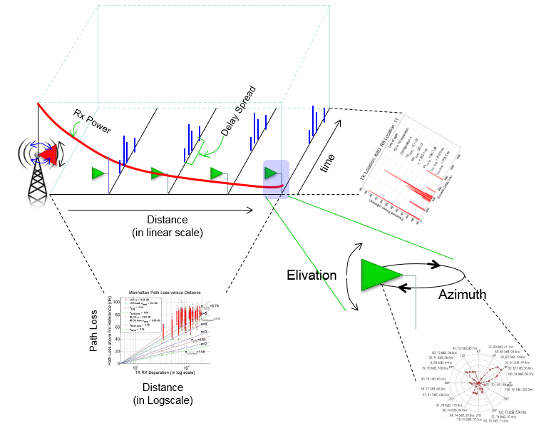
composite frame showing path loss, delay spread and angle of arrival on one set of axes

One sweep produces all three : a single measurement records power, arrival time and arrival angle together, which is why the three sit on one frame rather than coming from three separate experiments.
Each factor limits a different part of the receiver : path loss sets the link budget, delay spread sets the cyclic prefix and the equaliser, and angle of arrival sets what beamforming can recover.
The three insets are the same data replotted : they are three views of one channel, not three channels.
The list is deliberately short : Doppler and polarisation are absent from it, and the 3GPP model adds both.

Path Loss Modeling

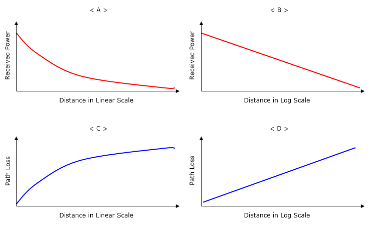
Path Loss between a Transmitter and Reciever can be best described by a plot. But you may see slightly different form of the plots from different papers and text books and sometimes those different representation may confuse you. So, it would be good to think of all the possible types of graph/plots before you reading papers and textbooks. I put the four different possible types which basically indicate the same physical properties but they are plotted a little different ways.

I think < A > would be the most straightfoward and intuitive representation. In this, the vertical axis represents the power measured by the receiver antenna and the horizontal axis represents the distance between Tx and Rx antenna in linear scale. By common sense and intuition, you would easily guess the received power will decrease as the distance gets larger. But how much the power get decreased ? Does it decrease by linear (straight line) fashion ? or some non linear (curve) fashion ? By high school physics, you may guess the power will decrease in anti-proportion to the distance squared. For more specifically, refer to Path Loss Model in Free Space. Now you can sense that the recieved power with distance would be something as in < A >.

< B > is telling the exactly same thing as < A > but you see the straight line not the curve. Why ? it is because the scale of the horizontal axis is Log scale. By nature (at least to me), Log scale does not looks natural.. but in some case converting it to linear scale is helpful to convert a nonlinear plot to linear plot and can process more easily in terms of statistics. Especially when you process measured data, linear fitting would be much easier than a curve fitting. So in many paper or textbook, you would see the plots represented as in < B >

< C > represents Path Loss with the distance between Tx and Rx. If you compare < A > and < C >, you would notice that they are complimentary. It is common sense. As Path Loss goes higher, the received power would goes lower. With the distance represented in linear scale, you see the Path Loss is plotted in non-linear (curve) pattern.

< D > is telling the exactly same thing as < C > but you see the straight line. This straight line is obtained by converting the horizontal scale (distance) to log scale.

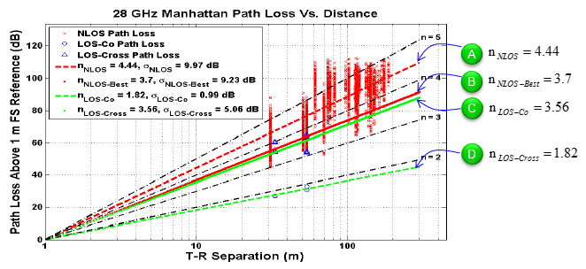
four plots of received power and path loss against distance in linear and log scale

Now let's look into the examples from real papers. One paper from NYU (Reference [2],[3]) shows following plot. This plot is based on type < D > described above. What you need to see from this graph is that the degree of Pass Loss change (Path Loss increase with the distance between Tx and Rx) changes depending on various situations.

28 GHz Manhattan path loss against T-R separation with fitted path loss exponents

< From Reference [2] [3] >

The four fitted exponents are the whole content of that plot, and the legend inside the axes is the one to read. The two non line of sight fits are n = 4.44 with a standard deviation of 9.97 dB, and n = 3.7 with 9.23 dB for the best pointing. The two line of sight fits are n = 1.82 with 0.99 dB on the matching polarisation, and n = 3.56 with 5.06 dB on the cross polarisation.

The green markers along the right hand edge carry the same four numbers, but on C and D the names are swapped with respect to that legend. Take the legend as correct. Line of sight on the matching polarisation is the case that should sit closest to free space, and 1.82 is just under the free space exponent of 2. The cross polarised measurement is both lossier and far less predictable, with a standard deviation five times larger. Assigning the numbers the other way round would put the much tighter 0.99 dB spread on the cross polarised case.

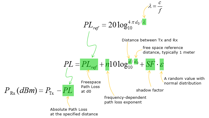
Once you have the plots from the measured data as shown above, you may be able to derive a certain mathematical model that explains the measured data. The mathematical model for the Path Loss for this plot is represented as shown below (This model came from Reference [2] and Matlab source code in Reference [1]). For the textbook style description/derivation of this model, refer to Path Loss Model in Real Situation : Shadowing.

path loss model equation with reference path loss, path loss exponent and shadow factor annotated

n (Path loss Exponent) : path loss exponent characterizes how the path loss increases with distance in a specific environment.

Environment Dependent: The value of n depends on the environment:

In free space, n is typically around 2.
In urban areas, n can range from 2.7 to 3.5 due to buildings and other obstructions.
In dense urban or indoor environments, n can be even higher, around 4 or more, due to multiple reflections, scattering, and absorption.

Impact on Path Loss: A higher value of n means the path loss increases more rapidly with distance. Consequently, the received signal power

P_Rx will decrease more quickly as the distance d from the transmitter increases.

SF(shadowing factor) : The shadowing factor SF · ε represents the variations in path loss caused by obstacles and environmental factors that are not captured by the basic distance-dependent path loss term. This component accounts for the random nature of the environment, which can cause fluctuations in the signal strength beyond the deterministic path loss.

SF: Shadowing Factor
- The shadowing factor SF is typically expressed in decibels (dB).
- It is a standard deviation of the log-normal distribution that models the variations in path loss due to shadowing.
- Commonly, SF ranges from 4 dB to 12 dB, depending on the environment.

ε: Random Variable
- ε is a Gaussian (normal) distributed random variable with a mean of 0 and a standard deviation of 1.
- This variable represents the randomness in the path loss due to shadowing effects.

Purpose of the Shadowing Factor

Capturing Environmental Variability:

The shadowing factor captures the impact of obstacles such as buildings, trees, and other objects that cause shadowing (also known as slow fading).
These obstacles can block or reflect the signal, causing additional path loss that varies randomly.

Realistic Path Loss Modeling:

Adding the shadowing term SF · ε to the path loss model makes it more realistic by accounting for the unpredictable nature of the environment.
This helps in accurately predicting signal coverage and quality in real-world scenarios.

Practical Example

Consider a scenario where a signal is transmitted in an urban environment with various buildings and other obstructions. The basic path loss model PL_ref + n · 10 log₁₀ (d / d₀) provides an average path loss based on distance. However, due to buildings and other obstacles, the actual path loss experienced by a receiver at a specific location can vary significantly. The shadowing factor SF · ε accounts for these variations:
If SF = 8 dB, it indicates a significant degree of shadowing.
The term SF · ε can add or subtract from the path loss, representing the random increase or decrease in signal strength due to shadowing.

Delay Spread

Path loss says how much of the transmitted power reaches the receiver. It says nothing about when that power arrives, and in a multipath channel it does not all arrive at once. Delay spread measures that scatter in time, and it is the property that decides how long a cyclic prefix has to be.

A property that represents a time domain nature of a channel is Delay Spread (See Delay Spread page if you are not familiar with the concept).

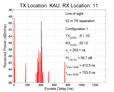
Following (Reference [2]) is the measurement of Delay Spread performed at a location 52 m away from the transmitter. As you see here, tau max (20 dB) is 753.5 ns which is equivalent to 226 m travel path. It implies that it is high degree of multi path environment.

power delay profile of a 52 m line of sight link with rms and threshold delay spreads

< From Reference [2] >

The annotations in the corner of that plot measure the same profile in three different ways, and the three answers are far apart. The rms delay spread is 203.1 ns. The excess delay at which the profile has fallen 10 dB below its peak is 412.5 ns, and the 20 dB delay is 753.5 ns. The link is line of sight over 52 m, with the transmitter pointed −5° in azimuth and −10° in elevation and the receiver at 20° and 0°.

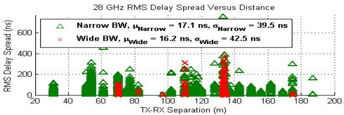
From Reference [3], you can get following plot showing the delay spread with various reciever locations.

28 GHz rms delay spread against T-R separation for narrow and wide bandwidth

< From Reference [3] >

The second plot changes what is being counted. Every marker is the rms delay spread of one link, plotted against transmitter to receiver separation from roughly 30 m out to 190 m. The narrow bandwidth measurements average 17.1 ns with a standard deviation of 39.5 ns, and the wide bandwidth measurements average 16.2 ns with a standard deviation of 42.5 ns. Measurement bandwidth therefore moved the result very little, which is the point the plot is making.

Reading the two plots together needs one caution. The 203.1 ns in the first is a single antenna pointing at one location, and the 17.1 ns in the second is an average over a whole campaign reported in a different paper. The first is not a typical value for this channel, and treating it as one would overstate the delay spread by more than an order of magnitude.

Three numbers describe one profile : the rms spread, the 10 dB delay and the 20 dB delay come from the same measurement and differ by nearly a factor of four.
The threshold measure is the pessimistic one : 753.5 ns of excess delay is 226 m of extra path, and that is the figure a cyclic prefix has to cover.
The rms value is the one the standard parameterises : 3GPP models delay spread as a log-normal variable and does not model the threshold delays at all.
The distribution is skewed : in both bandwidth cases the standard deviation is larger than the mean, so an average delay spread describes very few of the links it was averaged over.

Angle of Arrival

Power and timing together still leave the channel underdetermined. Two paths that arrive with the same delay and the same strength from opposite sides of the receiver are indistinguishable until the antenna is turned, and a beamforming system depends entirely on that difference. Angle of arrival is the measurement that separates them.

Another important property that shows the nature of a radio channel is Angle of Arrival. This can be obtained by measuring the recieived power while rotating the reciever antenna when the direction of transmission antenna is fixed.

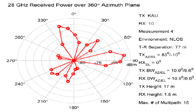
One example measurement from Reference [3] is as follows. You may notice there are several distinctive lobes here. This implies that there are several multipath that can play dominant roles in received signal.

28 GHz received power over the 360 degree azimuth plane on a non line of sight link

< From Reference 3 >

The conditions printed beside that plot set what it is able to resolve. The link is non line of sight over 77 m, with the transmitter 17 m up and the receiver at 1.5 m. Both antennas have a 10.9° azimuth beamwidth, so a full 360° sweep is about thirty three separate pointings rather than a continuous curve. The radial axis is received power in dBm, marked at −86, −76 and −66 dBm, and the annotation records a maximum of sixteen multipath components.

Following (Reference [5]) may not be directly related to 5G wave propogation, but I posted it here since it would give you a good idea on how to interpret the AoA plot shown above.

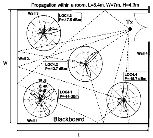
indoor room plan with four receiver locations and their azimuth power patterns

That indoor plot puts four polar patterns back into the room they were measured in. The room is 8.4 m long, 7 m wide and 4.3 m high, with the transmitter on wall 4 and four receiver locations spread across the floor. The received power is −14 dBm at LOC4.1, −12.7 dBm at LOC4.2, −17.5 dBm at LOC4.3 and −15.7 dBm at LOC4.4. The rings on each pattern are marked at 10, 20 and 30 dB. The dashed lines running from each location to the walls are the reflection paths, and each one lines up with a lobe on that location’s pattern.

That is why the indoor figure is here at all. The outdoor plot shows lobes without showing what produced them, and the indoor plot draws the reflecting surface next to each lobe. A lobe is a wall, or a building face, seen from the receiver.

Beamwidth is the resolution : a 10.9° beam cannot separate two paths closer together than that, so a lobe count is a lower bound on the number of paths rather than the number itself.
A lobe is a reflector : the indoor figure draws the path from each lobe back to the surface that made it.
None of these arrived directly : the outdoor link is non line of sight, so every component plotted reached the receiver by reflection.
Azimuth alone is half the measurement : the receiver elevation is fixed at 0° through the whole sweep, and the 3GPP model treats zenith arrival as a parameter of its own.

How this maps to the 3GPP channel model

Everything above is measurement. The industry also needed something a simulator could run, and it needed every company to run the same one, so measurements of this kind were turned into a specification. That document is TR 38.901, and the mapping from this page into it is direct, because the three factors named at the top are three of the parameters it generates.

TR 38.901 is titled Study on channel model for frequencies from 0.5 to 100 GHz, and the current version is v19.4.0. It started as TR 38.900, which covered 6 to 100 GHz, and was widened downward so that one document also covers the bands below 6 GHz. For system level simulation it defines urban microcell street canyon, urban macrocell, indoor office, rural macrocell, indoor factory and suburban macrocell.

Step 4 of its channel generation procedure is where this page connects to it. That step draws the large scale parameters as one correlated vector, written in the specification as [SF, K, DS, ASD, ASA, ZSD, ZSA]. Reading the abbreviations out, they are shadow fading, the Ricean K factor, rms delay spread, azimuth spread of departure, azimuth spread of arrival, zenith spread of departure and zenith spread of arrival. The three factors this page lists are SF, DS and ASA. They are not drawn independently either, because the cross correlations in Table 7.5-6 are imposed through a Cholesky decomposition before any of them is used.

Three differences between the model on this page and the one in the specification are worth knowing before any number is carried from one to the other.

The first is the reference distance. The formula above measures path loss from a free space value at d₀, typically 1 m, and that is exactly what 3GPP adopted. The study records the reason in its own words. The close-in free space reference replaced a floating optimisation parameter in order to provide a standard and stable definition of "path loss exponent" across all different parties, scenarios, and frequencies. Two groups fitting the same measurements with a free intercept obtain two different exponents, and pinning the intercept at 1 m removes that freedom.

The second is the distance itself. The formula above uses a single d. The specification uses the three dimensional separation d_3D, defined in Figure 7.4.1-1. For a terminal inside a building it splits the path further, into an outdoor and an indoor part, with d_2D-out, d_2D-in, d_3D-out and d_3D-in. The angle of arrival measurement above is a worked case. Its 77 m of ground separation, with the transmitter at 17 m and the receiver at 1.5 m, is 78.5 m in three dimensions. The gap widens as the terminal comes closer to the mast.

The third is the sign. The model above adds SF · ε to the path loss, so a positive draw means a weaker signal. A note under the specification’s parameter tables states the opposite convention. It reads the sign of the shadow fading is defined so that positive SF means more received power at UT than predicted by the path loss model. The draw is zero mean and symmetric, so no statistics are lost either way, but a value copied across without the flip is wrong.

The specification carries one thing this page does not, which is a rule for how the channel changes as a receiver moves a few metres. TR 38.901 makes shadow fading autocorrelated with distance through an exponential function whose correlation length depends on the environment, and clause 7.6.3 extends the same idea down to the cluster level as spatial consistency. A measurement campaign records fixed locations, so this is one place where the model had to supply something the measurements do not directly show.

The three factors here are three of seven : the specification generates SF, K, DS, ASD, ASA, ZSD and ZSA together. This page covers path loss, delay spread and azimuth arrival, and leaves the Ricean factor, the departure angles and the zenith angles to the specification.
The 1 m reference is the point of the model : it fixes the intercept so that a path loss exponent means the same thing wherever it was fitted. That is what makes the n = 4.44 above comparable with anyone else’s figure.
Use d_3D, not d : the specification measures the three dimensional separation, and splits outdoor from indoor for a terminal inside a building.
Check the sign of SF before reusing a value : positive means more received power in TR 38.901 and more loss in the formula above.
Correlation is the part a measurement does not give you : the autocorrelation of shadow fading and the spatial consistency procedure both exist for the same reason. A simulated terminal moving through a scenario has to see a channel that changes smoothly rather than one redrawn at every step.