As you know, a most typical approach to almost any of the engineering field is to draw out a mathematical model for each component of a system and combine all of the mathematical components to describe the whole system.
Let's assume that we built a mathematical model for each compoenent of a communication system as shown below. As you see, we have a mathematical model named as X which is the model for the signal from a transmitter. and we have another mathematical model named as Y which is for Recieved signal. and we have the model H which is for the channel.
As I described above, we have the mathematical model for each component of the system. Now the question is how do we combine these componend model to make it for the whole system ?
- Example - Calculation by Hand
- Identity
- Scaling
- Shifting
- Scaling and Shifting
- Reflection (Echo)
- Differentiator
- Integrator
- Exponential Decaying
- Some Funs with Sinosodial Signal and Convolution
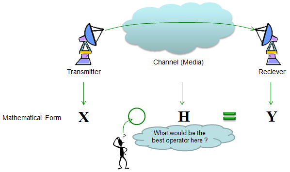
Partly by intuition and partly by our common sense, we would guess that 'combining X and Y in some format' should produce Y. Then the next question is 'How to combine X and Y' ?
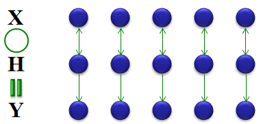
The first guess would be to try with basic operators like +,-,x,/. Let's think about basic property of these operation. My personal image of these operators are as shown below. Can you make any sense out of this ? Probably no. What I am trying to say with this illustration is "one lement of Y is created by only one element of X and only one element of H". Basically they are one to one operation. It means that a specific elements in Y is only influenced by only one specific elements in H and Y.
According to research and experiments, the received signal is not calculated by this kind of one-to-one operation as described above. In reality, one element in X is influenced by many other elements in X and Y. If I express this in an illustration, it would be as shown below.
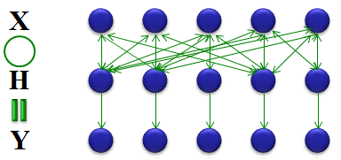
You might not haven't seen this kind of operation in high school math, but this kind of operation is very common to various engineering field and this would give you a lot of hard time at entering the university level engineering because you have never been familiar with this kind of operation in high school math.
The most commonly used operator which is operating like this is 'Convolution'. The convolution can be described as shown below. The symbol '*' represents 'Convolution'. (Don't get confused with multiplication symbol that you use in your computer software).
For further detailed description of Convolution, refer to Convolution section of Engineering Math.
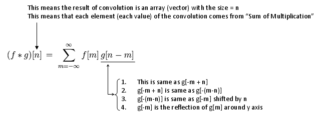
Convolution is a mathematical operator which gives the result when a sequence of a data goes through a specific process. Basically each elements of an output sequence is influenced by many previous element of input sequence and all the elements within the process the signal is going through. At the beginning, this would be very confusing cocept and just any of single explanation and lecture would never give you complete understanding for it. I am pretty sure that my explanation here would not give you the complete understanding if this is the first time for you to hear about 'Convolution', but if you have gone through many other resources before, i am pretty sure that my explanation would give you some additional insight and clarification. I stronly recomment you to try googling 'Convolution' and it would give you a lot of explanation with a little bit different aspects. You would find some Java applets or animation showing the concept of Counvolution. Even in YouTube, you would get a lot of lectures about Convolution. Try all those materials as much as possible.
Even though you have understandings of Convolution in mathematical sense, you would not have your own intuitive understandings of the concept without a lot of practice. Unlike the simple mathemtical operators like +,-,x,/ it would be very difficult to do practice about Convolution just by pen and paper since the calulation process is so complicated.
To help you with the practice, I would give you a short Matlab/Octave script. Try changing the vector x and chann and see how the outcome changes. Try to make your own association (relation) between input(x), chann and output(y).
- Example - Calculation by Hand
- Identity
- Scaling
- Shifting
- Scaling and Shifting
- Reflection (Echo)
- Differentiator
- Integrator
- Exponential Decaying
- Some Funs with Sinosodial Signal and Convolution
Example - Calculation by Hand
I strongly, strongly recommend you to try this on your own with pen and paper until you grasp the meaning of the process. (I posted the excel spreadsheet for this process. You can get it from here and try wth different values for f(n), g(n))

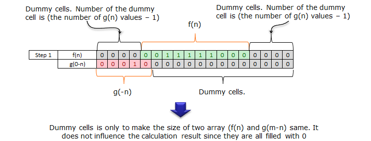
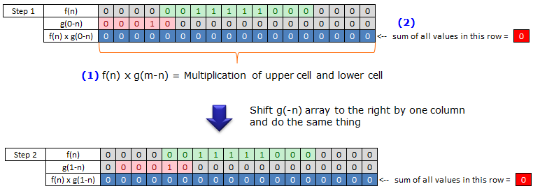
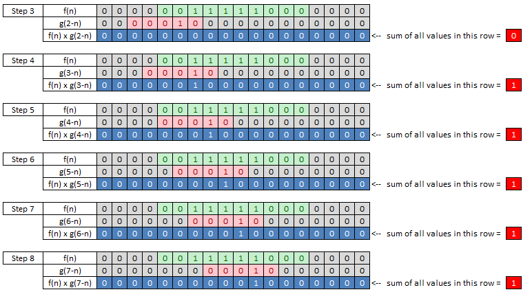
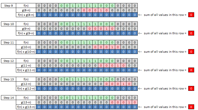
When you complete this whole process, collect the values shown in red cell on right side and place it in a raw from left to right. That is the final result of convolution.
If you think you got the complete understanding of the process shown above. Try followings by your hand and see if your answer is correct.

The steps above follow one procedure, and each row has a fixed job. The top row is f(n), the input, and it never moves. The middle row is the reversed channel, and it slides one column to the right at every step. The bottom row is the product of the two, taken cell by cell.
The number in the red box at the right of each step is the sum of that bottom row, and that single number is one sample of the output. Fourteen steps therefore produce fourteen output samples, which is why the answer is collected as a row rather than arrived at in one calculation.
The dummy cells at both ends exist only to make the two rows the same length. They hold zeros, so they contribute nothing to any product, and the count at each end is one less than the number of values in g(n).
The second example uses the same procedure with a wider channel. Here g(n) has four non zero taps instead of one, so the output is no longer a copy of the input. The rectangular input becomes a trapezoid, climbing through 1, 2, 3 to 4 and falling back the same way.
Identity
The sections from here on all use the same input and change only the channel. Starting from the simplest channel possible is what makes the comparison work, because every later result can be read as a departure from this one.
x = [0 1 0 1 0 1]; % Change this array if you want to change input sequence (transmitted data)
sf = 20; % samples per bit
p_x = x;
if sf > 1
for i = 2:sf
p_x= [p_x ; x];
end
p_x = reshape(p_x,[],1);
end
chan = [0 0 0 0 1 0 0 0 0 0]; % Change this array if you want to change the characteristics of channel
y = conv(p_x,chan);
subplot(2,5,[1 2]);stem(p_x);axis([1 length(p_x) -1.5 1.5]);title("tx signal");
subplot(2,5,3);stem(chan,'MarkerFaceColor',[0 0 1]);axis([1 length(chan) -1.5 1.5]);title("chan");
subplot(2,5,[4 5]);stem(y);axis([1 length(y) -1.5 1.5]);title("rx signal");
subplot(2,5,[6 7]);plot(p_x);axis([1 length(p_x) -1.5 1.5]);title("tx signal");
subplot(2,5,8);stem(chan,'MarkerFaceColor',[0 0 1]);axis([1 length(chan) -1.5 1.5]);title("chan");
subplot(2,5,[9 10]);plot(y);axis([1 length(y) -1.5 1.5]);title("rx signal");
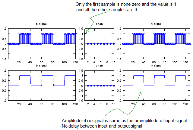
Now let's look at the first example. The input (tx signal) is a typtical rectangular pulse that you see in various electrical engineering books. The channel has 10 elements in it and only the first item is nonzero value 1 and all the other elements are set as '0'. Here the channel is a process which is manipulating the input sequence.
Look at the output. The output(rx signal) is the result of convolution of input(tx signal) and chan. You see there is no difference at all between the input and output. It means the channel in this example is just passing through the input sequence without any modification.
Scaling
Now let's look at another example. The input (tx signal) is a typtical rectangular pulse that you see in various electrical engineering books. The channel has 10 elements in it and only the first item is nonzero value 0.5 and all the other elements are set as '0'. Here the channel is a process which is manipulating the input sequence.
Look at the output. The output(rx signal) is the result of convolution of input(tx signal) and chan. You see there is no difference in terms of overall shape but the amplitude of output is half (0.5 times) of the input signal.
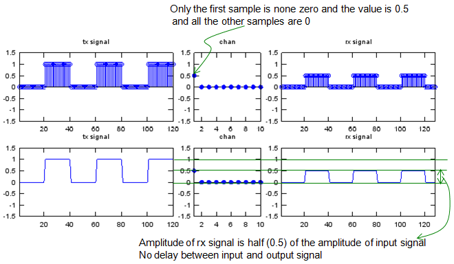
Only one number changed between this example and the one above. The single tap moved from 1 to 0.5, and the output amplitude followed it exactly.
That is the first of the two things a single tap can do. The value of the tap fixes the gain, and the gain applies to the whole signal rather than to part of it. The shape is untouched, which the lower right panel shows most clearly. The rectangular pulses keep their edges and their widths, and only their height changes.
In channel terms this is flat attenuation. A path that weakens a signal without spreading it in time produces exactly this, and it costs nothing but received power.
Shifting
Let's look at another example. The input (tx signal) is a typtical rectangular pulse that you see in various electrical engineering books. The channel has 10 elements in it and only the fifth is nonzero value 1 and all the other elements are set as '0'. This channel is almost same as the first example. The only difference is that the position for the non-zero value appears.
Look at the output. The output(rx signal) is the result of convolution of input(tx signal) and chan. You see there is almost no difference between the input and output and the only difference is that there is some delay between the input and output. It means the channel in this example is just delaying the input sequence without changing anything in terms of amplitude.
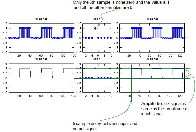
This time the tap kept its value and moved instead. It sits at sample 5 rather than at sample 1, and the output moved with it.
That is the second thing a single tap can do. The position of the tap fixes the delay, and the delay is the distance from the first sample to the tap. Five samples in gives five samples of delay out.
Nothing else changed. The amplitude matches the input and the pulse shape matches the input, so the output is the input rewritten later in time. A channel that only delays is harmless to the signal, and the receiver has only to know how far back to look.
Scaling and Shifting
Let's look at another example. The input (tx signal) is a typtical rectangular pulse that you see in various electrical engineering books. The channel has 10 elements in it and only the fifth is nonzero value 0.5 and all the other elements are set as '0'. This channel is almost same as the first example. The only difference is that the position for the non-zero value appears.
Look at the output. The output(rx signal) is the result of convolution of input(tx signal) and chan. Now you see two differences between the input and output. You would notice that both delay and amplitude has been changed. It means the channel in this example is just delaying the input sequence and changing the amplitude as well.
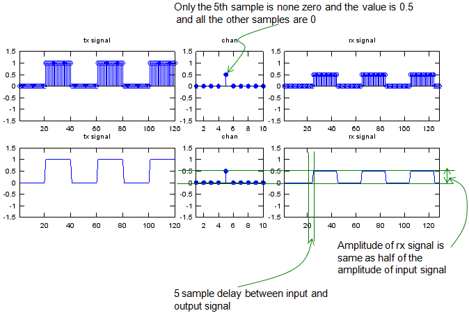
The two sections above changed one property each. This one changes both at once, with a tap of 0.5 sitting at sample 5.
The result is what those two results predict when put together. The output is delayed by five samples, exactly as in the shifting example, and its amplitude is half the input, exactly as in the scaling one. Neither effect disturbs the other.
That independence is the point of the series. A single tap carries two numbers, its position and its value, and each number controls a separate property of the output. Every channel in the sections below holds more than one tap, and each tap contributes its own delayed and scaled copy.
Reflection (Echo)
Every channel so far has had a single tap. A real radio path rarely does, because a signal that reaches the receiver directly also reaches it after bouncing off something. The channel below is the smallest model of that, with two taps instead of one.
x = [0 1 0 0 0 1 0 0 0];
sf = 20; % samples per bit
p_x = x;
if sf > 1
for i = 2:sf
p_x= [p_x ; x];
end
p_x = reshape(p_x,[],1);
end
chan = zeros(40,1);
chan(1) = 1;
chan(30) = 0.5;
y = conv(p_x,chan);
subplot(2,5,[1 2]);stem(p_x);axis([1 length(p_x) -1.5 1.5]);title("tx signal");
subplot(2,5,3);stem(chan,'MarkerFaceColor',[0 0 1]);axis([1 length(chan) -1.5 1.5]);title("chan");
subplot(2,5,[4 5]);stem(y);axis([1 length(y) -1.5 1.5]);title("rx signal");
subplot(2,5,[6 7]);plot(p_x);axis([1 length(p_x) -1.5 1.5]);title("tx signal");
subplot(2,5,8);stem(chan,'MarkerFaceColor',[0 0 1]);axis([1 length(chan) -1.5 1.5]);title("chan");
subplot(2,5,[9 10]);plot(y);axis([1 length(y) -1.5 1.5]);title("rx signal");
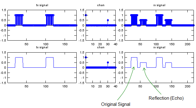
- The chan panel in the middle carries two taps. The first sits at sample 1 with a value of 1, and the second sits near sample 30 with a value of 0.5.
- The rx panel shows each input pulse twice. The first copy is labelled Original Signal and matches the input in height and in position.
- The second copy is labelled Reflection (Echo). It arrives about 30 samples later and stands at half the height, which is the position and the value of the second tap.
Nothing new is happening here. Each tap produces the delayed and scaled copy the sections above described, and the output is their sum. Two taps give two copies, and a channel with twenty taps would give twenty.
This is also the first example where the output runs longer than the input and where two copies can overlap. An echo arriving before the original pulse has finished adds to it sample by sample, and that overlap is what the last section on this page explores.
Differentiator
The two taps in this channel carry opposite signs, and that one change turns the channel into something that no longer resembles a propagation path. It earns a place here because it shows how much a two tap channel can do.
x = [0 1 0 1 0 1 0];
sf = 20; % samples per bit
p_x = x;
if sf > 1
for i = 2:sf
p_x= [p_x ; x];
end
p_x = reshape(p_x,[],1);
end
chan = [0 1 -1 0 0 0 0 0 0 0];
y = conv(p_x,chan);
subplot(2,5,[1 2]);stem(p_x);axis([1 length(p_x) -1.5 1.5]);title("tx signal");
subplot(2,5,3);stem(chan,'MarkerFaceColor',[0 0 1]);axis([1 length(chan) -1.5 1.5]);title("chan");
subplot(2,5,[4 5]);stem(y);axis([1 length(y) -1.5 15]);title("rx signal");
subplot(2,5,[6 7]);plot(p_x);axis([1 length(p_x) -1.5 1.5]);title("tx signal");
subplot(2,5,8);stem(chan,'MarkerFaceColor',[0 0 1]);axis([1 length(chan) -1.5 1.5]);title("chan");
subplot(2,5,[9 10]);plot(y);axis([1 length(y) -1.5 15]);title("rx signal");
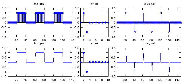
- The chan panel holds +1 at sample 2 and -1 at sample 3, so the channel subtracts each sample from the one before it.
- The rx panel is flat wherever the input is flat, because subtracting two equal samples gives zero.
- A spike appears at every edge of the input. A rising edge gives +1 and a falling edge gives -1, so the output marks where the input changed rather than what it was.
Subtracting the previous sample from the current one is a difference, and a difference is the discrete form of a derivative. That is where the section title comes from.
The practical reading is that taps of opposite sign remove whatever stays constant and keep whatever changes. A channel like this one passes edges and blocks steady levels, which is the behaviour of a high pass filter.
Integrator
The channel here holds many taps rather than two, and every one of them is positive and equal. Reversing the sign pattern of the section above produces the opposite behaviour.
x = [0 1 0 1 0 1 0];
sf = 20; % samples per bit
p_x = x;
if sf > 1
for i = 2:sf
p_x= [p_x ; x];
end
p_x = reshape(p_x,[],1);
end
chan = [0 1 1 1 1 1 1 1 1 1 1 1 1 1 1];
y = conv(p_x,chan);
subplot(2,5,[1 2]);stem(p_x);axis([1 length(p_x) -1.5 1.5]);title("tx signal");
subplot(2,5,3);stem(chan,'MarkerFaceColor',[0 0 1]);axis([1 length(chan) -1.5 1.5]);title("chan");
subplot(2,5,[4 5]);stem(y);axis([1 length(y) -1.5 15]);title("rx signal");
subplot(2,5,[6 7]);plot(p_x);axis([1 length(p_x) -1.5 1.5]);title("tx signal");
subplot(2,5,8);stem(chan,'MarkerFaceColor',[0 0 1]);axis([1 length(chan) -1.5 1.5]);title("chan");
subplot(2,5,[9 10]);plot(y);axis([1 length(y) -1.5 15]);title("rx signal");
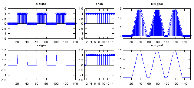
- The chan panel holds fifteen taps, and every one of them is 1.
- The rx panel no longer resembles the input. Each rectangular pulse becomes a ramp that rises, holds briefly and falls.
- The vertical scale changed as well. The output reaches about 14 rather than 1, because fifteen copies of the input are being added together.
Adding the last fifteen samples at every step is a running sum, and a running sum is the discrete form of an integral. That is where this section title comes from.
The two sections together frame the range. Taps of opposite sign gave a difference and passed only change, while taps of equal sign give a sum and pass only the average. A real channel sits between the two, and its tap pattern decides where.
Note : I posted a visual note in slideshow and animation format to show the concept of this example to give you more intuitive understanding. Check [Engineering]->[1]->[Convolution] in www.slide4math.com
Exponential Decaying
There would be no real system (no real channel) which is simple as simple as described above, but the example shown above would be a good example to help you understand very basic properties of Convolution.
Now I will give you some examples with a little bit more complicated channels.
x = [0 1 0 1 0 1]; % Change this array if you want to change input sequence (transmitted data)
sf = 20; % samples per bit
p_x = x;
if sf > 1
for i = 2:sf
p_x= [p_x ; x];
end
p_x = reshape(p_x,[],1);
end
a = 0.5;
t = 0:10;
k = 0.3;
chan = 0.5*exp(-k*t); % Try applying different functions here.
chan = [[0 0 0 0 0] chan]; % Change this array if you want to change the characteristics of channel
chan = chan/sum(chan);
y = conv(p_x,chan);
subplot(2,5,[1 2]);stem(p_x);axis([1 length(p_x) -1.5 1.5]);title("tx signal");
subplot(2,5,3);stem(chan,'MarkerFaceColor',[0 0 1]);axis([1 length(chan) -0.5 0.5]);title("chan");
subplot(2,5,[4 5]);stem(y);axis([1 length(y) -1.5 1.5]);title("rx signal");
subplot(2,5,[6 7]);plot(p_x);axis([1 length(p_x) -1.5 1.5]);title("tx signal");
subplot(2,5,8);stem(chan,'MarkerFaceColor',[0 0 1]);axis([1 length(chan) -0.5 0.5]);title("chan");
subplot(2,5,[9 10]);plot(y);axis([1 length(y) -1.5 1.5]);title("rx signal");
Note : I posted a visual note in slideshow and animation format to show the concept of this example to give you more intuitive understanding. Check [Engineering]->[1]->[Convolution] in www.slide4math.com
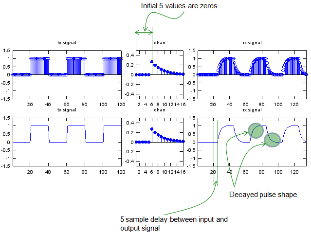
One simple example is as follows. As you see, the input is the same as the ones we used in previous examples. You would notice that the values in channel is much more complex than the ones we saw in previous examples. And the result is as shown below. If you already have gone through any basic electronic course, you would notice that the output is very similar to the case where a rectangular pulse is going through a capacitance circuit.
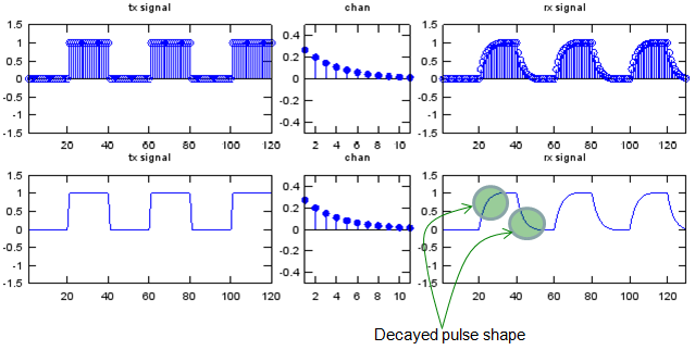
Let me give you another example. As you see, the input is the same as the ones we used in previous examples. You would notice that the values in channel is similar to previous example and the only difference is that you have some zeros at the beginning of channel sequence. And the result is as shown below. You see the overal shape of the output (rx signal) is same as the one you saw in previous example, but you would notice that a delay was introduced in this example.
Now I will give you even more complex examples. The Matlab/Octave code for these examples are listed below.
x = [0 1 0 1 0 1]; % Change this array if you want to change input sequence (transmitted data)
sf = 20; % samples per bit
p_x = x;
if sf > 1
for i = 2:sf
p_x= [p_x ; x];
end
p_x = reshape(p_x,[],1);
end
a = 0.5;
t = 0:10;
k = 0.3;
chan = 0.5*exp(-k*t).*cos(pi*t); % Try applying different functions here.
chan = [0 0 0 0 0 chan]; % Change this array if you want to change the characteristics of channel
chan = chan/chan(6);
y = conv(p_x,chan);
subplot(2,5,[1 2]);stem(p_x);axis([1 length(p_x) -1.5 1.5]);title("tx signal");
subplot(2,5,3);stem(chan,'MarkerFaceColor',[0 0 1]);axis([1 length(chan) -1.5 1.5]);title("chan");
subplot(2,5,[4 5]);stem(y);axis([1 length(y) -1.5 1.5]);title("rx signal");
subplot(2,5,[6 7]);plot(p_x);axis([1 length(p_x) -1.5 1.5]);title("tx signal");
subplot(2,5,8);stem(chan,'MarkerFaceColor',[0 0 1]);axis([1 length(chan) -1.5 1.5]);title("chan");
subplot(2,5,[9 10]);plot(y);axis([1 length(y) -1.5 1.5]);title("rx signal");
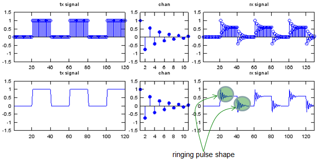
Let me give you an example. As you see, the input is the same as the ones we used in previous examples. You would notice that the values in channel is similar to previous example and the difference is that we have both positive and negative values alternating each ofther in channel sequence. And the result is as shown below. You see the ringing both at rising and falling phase. This is a very similar case where a signal is going through a L-C circuit or typical transmission lines.
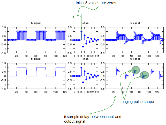
Let me give you another example. As you see, the input is the same as the ones we used in previous examples. You would notice that the values in channel is similar to previous example and the only difference is that you have some zeros at the beginning of channel sequence. And the result is as shown below. You see the overal shape of the output (rx signal) is same as the one you saw in previous example, but you would notice that a delay was introduced in this example.
Note : I posted a visual note in slideshow and animation format to show the concept of this example to give you more intuitive understanding. Check [Engineering]->[1]->[Convolution] in www.slide4math.com
Some Funs with Sinosodial Signal and Convolution
Every example so far has used a rectangular input, where a delayed copy is easy to pick out by eye. A sinusoid behaves differently. A delayed sinusoid is still a sinusoid at the same frequency, so the two copies add into one wave rather than sitting side by side.
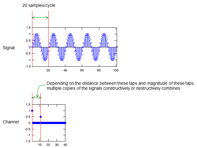
The drawing above sets the scene rather than showing a result. The signal at the top runs at 20 samples per cycle, and the channel below it has two taps, one at the start and one near sample 10. The note points at the distance between those taps, because that distance decides whether the two copies reinforce each other or cancel.
- The signal is the same 20 samples per cycle sinusoid, and the channel has a tap of 1 at the start with a tap of 0.5 ten samples later.
- Ten samples is half a cycle at this frequency, so the delayed copy arrives exactly out of phase with the original.
- The rx panel is therefore smaller than the tx panel. The two copies subtract rather than add, and the amplitude falls towards the difference between the two tap values.
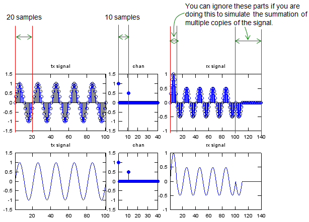
The marked regions at the left and the right are edge effects. They cover the part of the output where the two copies do not fully overlap, and the note above the figure says to ignore them.
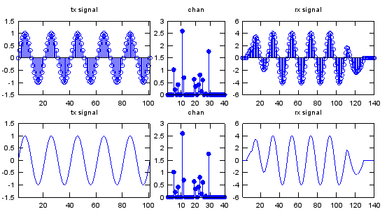
The figure above replaces those two taps with many, at scattered positions and heights. The output is still a sinusoid at the same frequency, because a sum of delayed sinusoids is one, but its amplitude has grown past 4 and its first cycle takes a while to settle.
The settling is the same edge effect as above. The amplitude is the sum of every tap contribution once the phases are accounted for, so a channel that builds one frequency up this way will cancel another. That is frequency selective fading written as a convolution.
SamplesPerCycle = 20;
x = 0:2*pi/SamplesPerCycle:10*pi;
p_x = sin(x);
chan = zeros(1,2*SamplesPerCycle);
chan(1) = 1;
chan(SamplesPerCycle/2+1) = 0.5;
y = conv(p_x,chan);
subplot(2,5,[1 2]);stem(p_x);axis([1 length(p_x) -1.5 1.5]);title("tx signal");
subplot(2,5,3);stem(chan,'MarkerFaceColor',[0 0 1]);axis([1 length(chan) -1.5 1.5]);title("chan");
subplot(2,5,[4 5]);stem(y);xlim([1 length(y)]);title("rx signal");
subplot(2,5,[6 7]);plot(p_x);axis([1 length(p_x) -1.5 1.5]);title("tx signal");
subplot(2,5,8);stem(chan,'MarkerFaceColor',[0 0 1]);axis([1 length(chan) -1.5 1.5]);title("chan");
subplot(2,5,[9 10]);plot(y);xlim([1 length(y)]);title("rx signal");