Exponential Function

I think one of the most famous mathematical term in both science and engineering is 'exponential' which is represented as follows. Every example on this page comes from this one form. Only the value of k changes, or several terms of this form are added or multiplied together.

Exponential function e to the power k t

The purpose of this page is to give you some intuitive understanding of various exponential form and I recommend you to try to visualize any equations or formula which is made up of this component.

I will put various examples as much as possible in this page. You may use this page as a small dictionary for exponential function. Whenever you see any exponential function while you are reading literature, get back to this page and see how it look like.

The page moves in three steps. The first sections change the type of k: real, imaginary and complex. The middle sections show the form inside three probability distributions: Normal, Log Normal and Rayleigh. The last sections show solutions of differential equations and step responses of transfer functions, which are sums and products of such terms.

When k is a 'real' number
When k is an 'imaginary' number and the real part of the complex number is '0'
Combination of case 1 and Case 2 - Multiplying Case 1 and Case 2
Euler form of a Complex Number : Exponential Function to represent a Complex Number
When the k is a complex number
Representation of Signal
Probablistic Distribution Function

Solution of Differential Equation

Transfer Functions

Note : For more intuitive understandings on the concept of Exponential function and application, I posted another types of note mainly in the form of various graphs at www.freetechslide.com.

When k is a 'real' number

This is easy to understand. When the k is a real number, you would have a plot with t as follows. (left plot is the case when k is positive value and the right plot is the one when k is negative value).

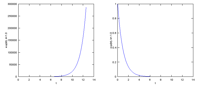
Exponential function e to the power k t

Plots of exp of k t for k equal to 1.0 and k equal to -1.0

With a positive k the curve grows without limit, and with a negative k it decays toward zero.

k sets the rate, not only the direction : the left plot uses k = 1.0 and the right plot uses k = -1.0. At t = 4π, about 12.57, the left curve reaches e^12.57, which is about 287,000. That is why the curve looks flat until t = 8 and then rises steeply.
A negative k gives a time constant : with k = -1.0 the curve falls to e^-1, about 0.37, at t = 1. It is about 1% of its start value at t = 4.6. In general, the value drops to 37% of itself every 1/|k| seconds.
Every curve starts at 1 : e⁰ = 1 for any k, so both plots pass through the value 1 at t = 0. Only the slope at that point, which equals k, is different.
The rate of change is proportional to the value : the slope of e^kt is k e^kt. This is why e^kt is the solution of y' = k y, and why it appears in every later section of this page.

See this page for slideshow on this function. You would see more generic description on this form of exponential function,

When k is an 'imaginary' number and the real part of the complex number is '0'

This is the case where the equation is represented as e^(i t). As you see in the following plot, suprisinly this form can represent a cyclic (periodic) behaviour. (You would be able to find mathematical ground on how e^(i t) can represent the periodic behaviour.) This would be one of the most important and widely used form of exponential function. See Euler Form section in Complex Number pages to find how the exponential function can represent the cyclic behaviour.

Unit circle trajectory of exp of j k t with its real and imaginary parts against t

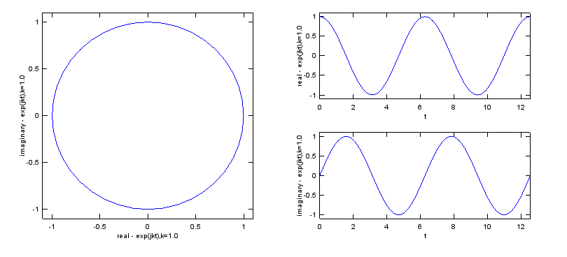
The point e^it moves around the unit circle, so its real part is cos t and its imaginary part is sin t.

The magnitude never changes : |e^it| = 1 for every t, so the trajectory on the left stays on the circle of radius 1. Nothing grows and nothing decays.
One turn takes 2π : the right plots run from t = 0 to 4π, about 12.57, so each of them shows exactly two periods. The labels in the plot write the exponent as jkt with k = 1.0, which is the same function.
The imaginary part lags by a quarter period : the real part starts at 1 and the imaginary part starts at 0. The sine reaches its peak at t = π/2, a quarter turn after the cosine.
i and j are the same symbol : mathematics writes i for the imaginary unit. Engineering texts and Matlab write j, because i is often used for current.

See this page for slideshow on this function. You would see the step by step procedure of producing this plot,

Combination of case 1 and Case 2 - Multiplying Case 1 and Case 2

If you simply multiplying the case 1 and case 2, you would be able to get the following result. As you see, now you can represent spiraling (cyclic + damping or cyclic + magnifying). Mathematical format of these are as follows.

Understanding this form is very important when you try to evaluate 'stability of a transfer function' in control system or filter design.

Following is the case when k is smaller than 0.

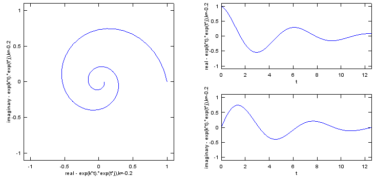
Inward spiral of exp of k t times exp of j t for k equal to -0.2

With k = -0.2 the point circles and moves inward, so the trajectory is a spiral toward the origin.

The radius is e^kt : |e^kt e^it| = e^kt, because |e^it| = 1. So the real exponential sets the radius, and the imaginary one sets the angle.
Each turn shrinks the radius by the same factor : one turn takes 2π, so the radius is multiplied by e^{-0.2 x 2π}, about 0.28, on every turn. Each loop of the spiral is a little more than a quarter of the size of the loop before it.

Following is the case when k is greater than 0.

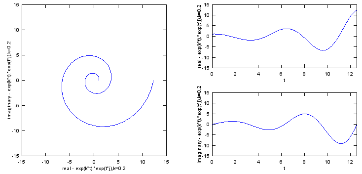
Outward spiral of exp of k t times exp of j t for k equal to 0.2

With k = 0.2 the same rotation grows outward, and after two turns the radius is e^0.8π, about 12.3.

The sign of k decides stability : a negative k gives a spiral that settles at 0, and a positive k gives one that grows without limit. For a transfer function, the same test applies to each pole: its real part must be negative.
The time plots are a cosine and a sine inside an envelope : e^kt e^it = e^kt cos t + i e^kt sin t. So the right-hand plots stay between the two curves +e^kt and -e^kt.

See this page and this page for slideshow on this function. You would see more generic description on this form of exponential function,

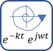
Euler form of a Complex Number : Exponential Function to represent a Complex Number

Exponential function can be used as a way to represent a complex number as shown below. This type of presentation for a complex number is called 'Euler form'. See here for the detailed explanation.

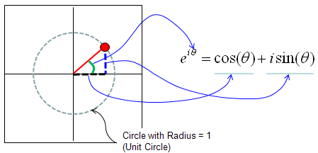
Unit circle with angle theta and Euler equation e to the i theta equals cos theta plus i sin theta

The angle θ on the unit circle sets both parts of e^iθ: cos θ is the horizontal side and sin θ is the vertical side.

Any complex number is a scaled point on this circle : a complex number z = x + iy is written z = r e^iθ. Here r = sqrt(x² + y²) is the magnitude, and θ is the angle from the positive real axis.
Multiplication adds the angles : r₁e^iθ1 x r₂e^iθ2 = r₁r₂e^{i(θ1 + θ2)}. This is the main reason engineers use the Euler form for rotation and phase shift.
A worked value : at θ = π, cos π = -1 and sin π = 0, so e^iπ = -1.

The diagram below samples the circle at 40 equal angles. Each red dot is e^(n/40)2πi for n = 0 to 39, so neighbouring dots are 2π/40 apart. That is about 0.157 rad, or 9 deg.

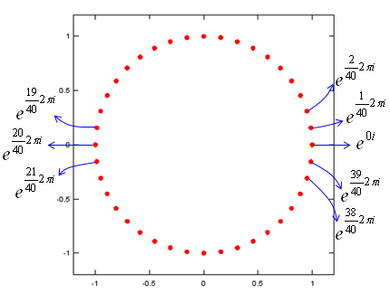
Forty points of e to the power n over 40 times 2 pi i on the unit circle

Equal steps in the exponent move the point around the circle by equal angles, and n = 40 returns to e⁰ⁱ = 1.

The labels climb counterclockwise : e⁰ⁱ sits at 1 on the right. The labels 1/40 and 2/40 are just above it, and 39/40 and 38/40 are just below it.
The label 20/40 sits at -1 : e^(20/40)2πi = e^iπ = -1, which is the dot on the negative real axis. The labels 19/40 and 21/40 are its two neighbours.

See this page for slideshow on this function. You would see more generic description on this form of exponential function,

When the k is a complex number

This example represent the following format. This is basically the same form as the one we saw in previous case. It is just a little bit different mathematical presentation.

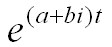
This case represent the form e^((a + b i) t) and depending on a, b you would have following different results. I think this is the most important form and you will see this form in almost every area of engineering. Fourier Transform, Differential Equation, Control System Design, Filter Design are only a portion of examples.

I strongly recommend you to have very concrete understanding of this form. Trying with various a, b values and see if how the result changes in the matlab code listed below can be a great help.

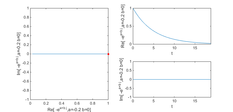
Following case is when a = -0.2, b = 0.0; Since imaginary part does not exists you don't see any oscillation trajectory. Since real part is negative value, the amplitude of the trajectory decreases as time goes on.

NOTE : The red poin in the plot indicates the starting point of the trajectory.

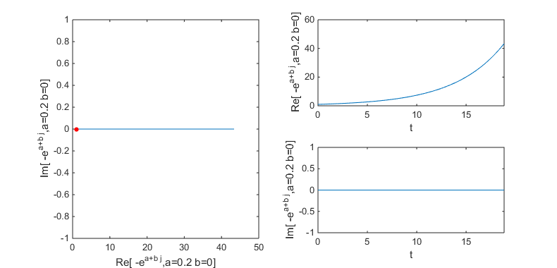
Trajectory and real and imaginary parts for a equal to -0.2 and b equal to 0

Following case is when a = 0.2, b = 0.0; Since imaginary part does not exists you don't see any oscillation trajectory. Since real part is a positive value, the amplitude of the trajectory increases as time goes on.

NOTE : The red poin in the plot indicates the starting point of the trajectory.

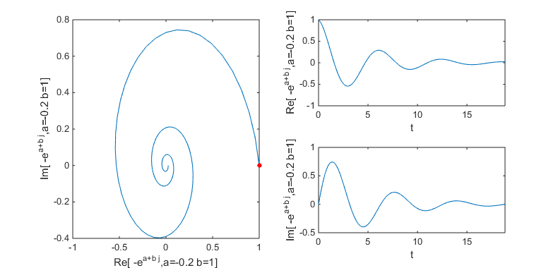
Trajectory and real and imaginary parts for a equal to 0.2 and b equal to 0

Following case is when a = -0.2, b = 1.0; Since imaginary part exists you see oscillation trajectory. Since real part is a negative value, the amplitude of the trajectory decreases as time goes on.

NOTE : The red poin in the plot indicates the starting point of the trajectory.

Inward spiral and damped real and imaginary parts for a equal to -0.2 and b equal to 1

Following case is when a = 0.2, b = 1.0; Since imaginary part exists you see oscillation trajectory. Since real part is a positive value, the amplitude of the trajectory increases as time goes on.

NOTE : The red poin in the plot indicates the starting point of the trajectory.

Outward spiral and growing real and imaginary parts for a equal to 0.2 and b equal to 1

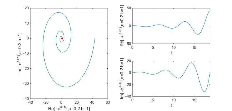
Following case is when a = -0.2, b = 2.0; Since imaginary part exists you see oscillation trajectory. The coefficient of imaginary part(b) is greater than in the previous example and you see the oscillation with higher frequency. Since real part is a negative value, the amplitude of the trajectory decreases as time goes on.

NOTE : The red poin in the plot indicates the starting point of the trajectory.

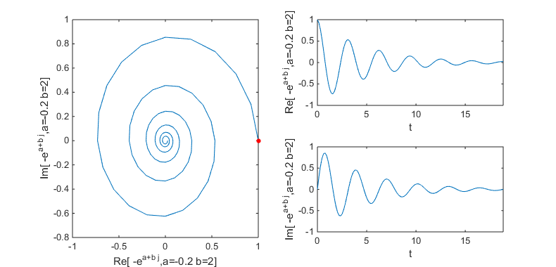
Inward spiral and damped real and imaginary parts for a equal to -0.2 and b equal to 2

The real part a sets the envelope and the imaginary part b sets the rotation speed. The two parameters act independently.

The envelope is e^at : the code runs t from 0 to 6π, about 18.85. So a = -0.2 ends at e^{-0.2 x 6π}, about 0.023, and a = 0.2 ends at about 43.4. That end value is where the a = 0.2 plots stop on the real axis.
b is the angular frequency : one turn takes 2π/b. With b = 1 the plot shows three turns over 6π, and with b = 2 it shows six.
The b = 2 spiral has corners : the step 2*pi/40 gives only 20 samples per turn when b = 2. The plot joins the samples with straight lines, so the curve looks like a polygon. A smaller step, such as 2*pi/400, gives a smooth spiral.
Every trajectory starts at 1 : e⁰ = 1 for any a and b, so the red dot always sits at the point 1 + 0j. In the a = 0.2 plots it looks close to the origin only because the axes reach 40.

Can you identify the characteristics of variable a (real part of the complex number) and b(imaginary part of the complex number) ? Try with the following matlab code. You can change the value of a,b to get the examples shown above.

t=0:2*pi/40:6*pi;
a = 0.2;
b = 1.0;
f = exp((a+b*j)*t);

subplot(2,2,[1 3]);
plot(real(f),imag(f));
hold on
plot(real(f(1)),imag(f(1)),'ro','MarkerFaceColor',[1 0 0],'MarkerSize',4)
hold off
xlabel(strcat('Re[ -e^{a+b j},a=',num2str(a),' b=',num2str(b),']'));
ylabel(strcat('Im[ -e^{a+b j},a=',num2str(a),' b=',num2str(b),']'));

subplot(2,2,2);
plot(t,real(f));
xlim([0 max(t)]);
xlabel('t');
ylabel(strcat('Re[ -e^{a+b j},a=',num2str(a),' b=',num2str(b),']'));

subplot(2,2,4);
plot(t,imag(f));
xlim([0 max(t)]);
xlabel('t');
ylabel(strcat('Im[ -e^{a+b j},a=',num2str(a),' b=',num2str(b),']'));

set(gcf, 'Position', [100 100 790 380]);

One detail in the listing is worth knowing before you change it. The axis labels print -e^{a+b j}, but the code plots exp((a+b*j)*t). The plotted function has no minus sign, and its exponent includes t. The labels are text only, so the plots themselves are correct.

Representation of Signal

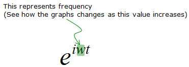
A signal in communication is often written as e^iωt, where ω is the angular frequency in rad/s. This is the e^it form of the earlier section, with the rotation speed written out. Let's see what changes when ω increases.

e to the power i omega t with omega marked as the frequency

The plots below show the real part and the imaginary part for ω = 1, 2, 3 and 4. Every plot covers the same interval, from 0 to 2π.

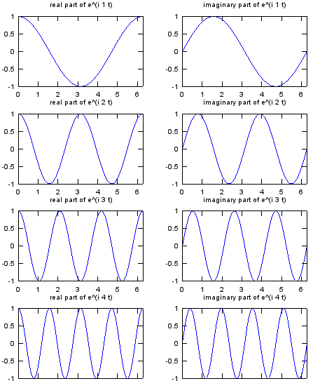
Real and imaginary parts of e to the power i omega t for omega from 1 to 4

Each step up in ω adds one more full cycle inside the same interval of 2π.

ω counts cycles per 2π : the row for ω = 3 shows three full cycles between 0 and 2π. In general, the period is 2π/ω, and the frequency in Hz is f = ω/2π.
The real part is a cosine and the imaginary part is a sine : e^iωt = cos ωt + i sin ωt. So the left column shows cos ωt and the right column shows sin ωt.
A negative ω is a real frequency too : e^-iωt turns clockwise. The sum e^iωt + e^-iωt is 2 cos ωt. This is why the spectrum of a real cosine has two lines, one at +ω and one at -ω.
The listing computes one case more than it plots : it builds exp_iwt_5 for ω = 5, but the 4x2 subplot grid has room only for ω = 1 to 4. So ω = 5 is not shown.

t = 0:pi/100:2*pi;

w = 1;
exp_iwt_1 = exp(j .* w .* t);

w = 2;
exp_iwt_2 = exp(j .* w .* t);

w = 3;
exp_iwt_3 = exp(j .* w .* t);

w = 4;
exp_iwt_4 = exp(j .* w .* t);

w = 5;
exp_iwt_5 = exp(j .* w .* t);


subplot(4,2,1);
plot(t,real(exp_iwt_1)); xlim([0 2*pi]); title('real part of e^(i 1 t)');
subplot(4,2,2);
plot(t,imag(exp_iwt_1)); xlim([0 2*pi]); title('imaginary part of e^(i 1 t)');

subplot(4,2,3);
plot(t,real(exp_iwt_2)); xlim([0 2*pi]); title('real part of e^(i 2 t)');
subplot(4,2,4);
plot(t,imag(exp_iwt_2)); xlim([0 2*pi]); title('imaginary part of e^(i 2 t)');

subplot(4,2,5);
plot(t,real(exp_iwt_3)); xlim([0 2*pi]); title('real part of e^(i 3 t)');
subplot(4,2,6);
plot(t,imag(exp_iwt_3)); xlim([0 2*pi]); title('imaginary part of e^(i 3 t)');

subplot(4,2,7);
plot(t,real(exp_iwt_4)); xlim([0 2*pi]); title('real part of e^(i 4 t)');
subplot(4,2,8);
plot(t,imag(exp_iwt_4)); xlim([0 2*pi]); title('imaginary part of e^(i 4 t)');

Normal Distribution

The bell curve describes a quantity that gathers around one value. Small deviations from that value are common, and large ones are rare. Thermal noise in a receiver is the standard example in communication.

Another very popular application of exponential form is in Statistics and various kind of probablistic distribution is represented as a exponential form.

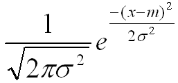
Normal distribution formula with mean m and standard deviation sigma

The most typical example is 'Normal Distribution' (Bell Shaped distribution) as follows.

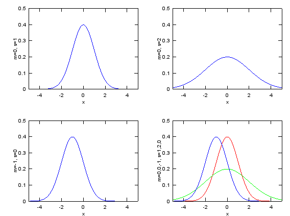
Normal distribution curves for three combinations of m and sigma

Changing m moves the bell along x, and a larger σ widens the bell and lowers its peak.

The exponent does the shaping : -(x - m)²/(2σ²) is 0 at x = m and becomes more negative with the square of the distance from m. The factor in front only scales the total area to 1.
The peak height is 1/sqrt(2πσ²) : this is about 0.399 for σ = 1 and about 0.199 for σ = 2. The area under every curve stays 1, so a wider curve must be lower.
m shifts the curve and σ scales it : the lower left plot has m = -1, so its peak sits at x = -1. Its shape is the same as the upper left curve.
One label in the listing is wrong : the code writes σ as s. It sets s = 1 for e3, but the label says 'm=-1, s=0', and the combined plot says 's=1,2,0'. A normal distribution with σ = 0 is not defined. The curve drawn is the σ = 1 case, and its 0.399 peak confirms it.
Colours in the combined plot : red is m = 0, σ = 1. Green is m = 0, σ = 2. Blue is m = -1, σ = 1.

x=-5:0.02:5;
m = 0;
s = 1;
e1 = 1/sqrt(2*pi*s^2)*exp(-(x-m).^2/(2*s^2));
m = 0;
s = 2;
e2 = 1/sqrt(2*pi*s^2)*exp(-(x-m).^2/(2*s^2));
m = -1;
s = 1;
e3 = 1/sqrt(2*pi*s^2)*exp(-(x-m).^2/(2*s^2));

subplot(2,2,1);plot(x,e1);axis([-5 5 0 0.5]);xlabel('x');ylabel('m=0, s=1');
subplot(2,2,2);plot(x,e2);axis([-5 5 0 0.5]);xlabel('x');ylabel('m=0, s=2');
subplot(2,2,3);plot(x,e3);axis([-5 5 0 0.5]);xlabel('x');ylabel('m=-1, s=0');
subplot(2,2,4);plot(x,e1,'r-',x,e2,'g-',x,e3,'b-');axis([-5 5 0 0.5]);xlabel('x');ylabel('m=0,0,-1, s=1,2,0');

See this page for slideshow on this function. You would see more generic description on this form of exponential function,

Log Normal Distribution

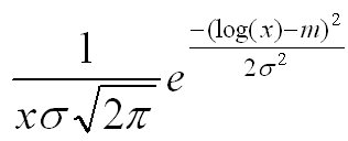
Try to find what is the difference between this form and Normal distribution just by looking at the mathematical presentation. You will find the two major difference.

i) log(x) is used in stead of 'x' (horizontal axis become log scale and by definition of log, this function can be used only when x > 0

ii) 1/x (decreasing function) is multiplied with the exponential term.

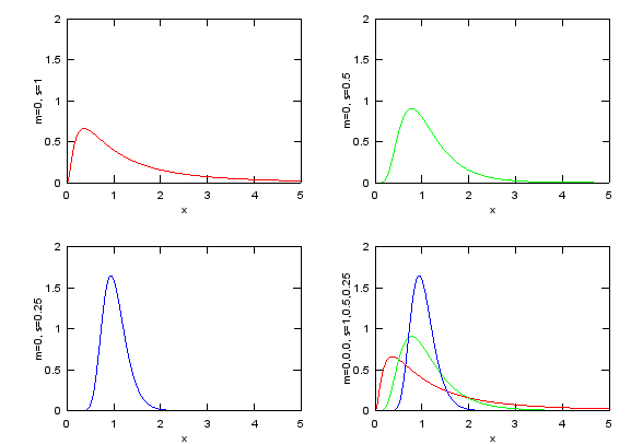
Log normal distribution formula with log x in place of x and a 1 over x factor

Log normal distribution curves for sigma equal to 1, 0.5 and 0.25

The log normal curve starts at 0 at x = 0, rises to a single peak and has a long tail to the right.

ln x is normal : if a variable X follows this distribution, ln X follows the normal distribution with mean m and standard deviation σ. That is the meaning of the name. The function log in Matlab and Octave is the natural logarithm ln.
The peak sits at e^{m - σ²} : with m = 0 this is about 0.37 for σ = 1, 0.78 for σ = 0.5 and 0.94 for σ = 0.25. The peak heights are about 0.66, 0.90 and 1.65, and they match the three plots.
The median stays at e^m = 1 : all three curves have half of their area to the left of x = 1. The mean is e^{m + σ²/2}, about 1.65 for σ = 1. The long right tail pulls the mean above the median.
The curve starts at 0 despite the 1/x factor : near x = 0 the exponential part falls faster than 1/x grows, so the product goes to 0.

x=0:0.02:5;
m = 0;
s = 1;
e1 = 1./(x.*s*sqrt(2*pi)).*exp(-(log(x)-m).^2/(2*s^2));
m = 0;
s = 0.5;
e2 = 1./(x.*s*sqrt(2*pi)).*exp(-(log(x)-m).^2/(2*s^2));
m = 0;
s = 0.25;
e3 = 1./(x.*s*sqrt(2*pi)).*exp(-(log(x)-m).^2/(2*s^2));

subplot(2,2,1);plot(x,e1,'r-');axis([0 5 0 2]);xlabel('x');ylabel('m=0, s=1');
subplot(2,2,2);plot(x,e2,'g-');axis([0 5 0 2]);xlabel('x');ylabel('m=0, s=0.5');
subplot(2,2,3);plot(x,e3,'b-');axis([0 5 0 2]);xlabel('x');ylabel('m=0, s=0.25');
subplot(2,2,4);plot(x,e1,'r-',x,e2,'g-',x,e3,'b-');axis([0 5 0 2]);xlabel('x');ylabel('m=0,0,0, s=1,0.5,0.25');

See this page for slideshow on this function. You would see more generic description on this form of exponential function,

Rayleigh Distribution

This form of distribution is very widely used for channel modeling in wireless communication. You will not be able to understanding anything about 'Fading' without understanding this function.

Try to find the difference between this form and Normal distribution and try to find the common part as well.

i) there is no 'm' (mean) term in the equation. (It means the 'mean' of the underlying Gaussian components is assumed to be '0')

ii) the exponential function part is exactly same as 'Normal Distribution with m = 0'

iii) x (increasing function) is multiplied to the exponential function.

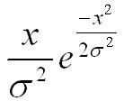
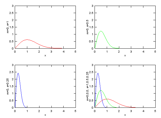
Rayleigh distribution formula x over sigma squared times exp of minus x squared over 2 sigma squared

Rayleigh distribution curves for sigma equal to 1, 0.5 and 0.25

The Rayleigh curve starts at 0, peaks at x = σ and has a tail to the right.

It is the magnitude of two Gaussian components : take two independent Gaussian variables X and Y, each with mean 0 and standard deviation σ. The magnitude R = sqrt(X² + Y²) follows this distribution. In a fading channel, X and Y are the in-phase and quadrature parts of many scattered paths, and R is the envelope of the received signal.
The peak is at x = σ : the peak height is e^-1/2/σ. That is about 0.61, 1.21 and 2.43 for σ = 1, 0.5 and 0.25, and it matches the three plots.
The mean of R is not zero : the mean is σ sqrt(π/2), about 1.25σ. The zero mean belongs to X and Y, not to R.
The m lines in the listing have no effect : the code sets m = 0 for each curve, but the Rayleigh formula has no m. So those lines do not change the result.

x=0:0.02:5;
m = 0;
s = 1;
e1 = x./(s^2).*exp(-(x.^2)/(2*s^2));
m = 0;
s = 0.5;
e2 = x./(s^2).*exp(-(x.^2)/(2*s^2));
m = 0;
s = 0.25;
e3 = x./(s^2).*exp(-(x.^2)/(2*s^2));

subplot(2,2,1);plot(x,e1,'r-');axis([0 5 0 3]);xlabel('x');ylabel('m=0, s=1');
subplot(2,2,2);plot(x,e2,'g-');axis([0 5 0 3]);xlabel('x');ylabel('m=0, s=0.5');
subplot(2,2,3);plot(x,e3,'b-');axis([0 5 0 3]);xlabel('x');ylabel('m=0, s=0.25');
subplot(2,2,4);plot(x,e1,'r-',x,e2,'g-',x,e3,'b-');axis([0 5 0 3]);xlabel('x');ylabel('m=0,0,0, s=1,0.5,0.25');

See this page for slideshow on this function. You would see more generic description on this form of exponential function,

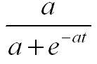
Sigmoid : a/(a + e^-at)

A population cannot grow exponentially forever, because food and space are limited. The sigmoid, or logistic, curve adds that limit. It grows like an exponential at first, and then it approaches 1 and stays there.

This example represent the following form. This form is frequently used for the mathemtical modeling for population growth and chemical reaction etc.

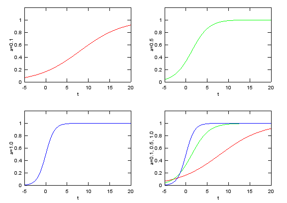
Sigmoid formula a over a plus e to the power minus a t

Sigmoid curves for three values of a

A larger a gives a steeper rise, and every curve approaches the same limit of 1.

It solves the logistic equation : y = a/(a + e^-at) satisfies y' = a y (1 - y). When y is small, y' is close to a y, which is exponential growth. When y is close to 1, the factor 1 - y stops the growth.
The start value depends on a : at t = 0 the curve is a/(a + 1). That is about 0.17 for a = 0.2, 0.33 for a = 0.5 and 0.5 for a = 1.0.
The midpoint moves with a : y = 0.5 when e^-at = a, that is at t = ln(1/a)/a. This gives t = 8.0 for a = 0.2, t = 1.4 for a = 0.5 and t = 0 for a = 1.0.
One label does not match the code : the code sets a = 0.2 for e1, but the plot labels say a=0.1. The red curve starts at about 0.17, which is the a = 0.2 value. So the label is the part that is wrong.

t=-5:0.02:20;
a = 0.2;
e1 = a./(a.+exp(-a.*t));
a = 0.5;
e2 = a./(a.+exp(-a.*t));
a = 1.0;
e3 = a./(a.+exp(-a.*t));

subplot(2,2,1);plot(t,e1,'r-');axis([t(1) t(end) 0 1.2]);xlabel('t');ylabel('a=0.1');
subplot(2,2,2);plot(t,e2,'g-');axis([t(1) t(end) 0 1.2]);xlabel('t');ylabel('a=0.5');
subplot(2,2,3);plot(t,e3,'b-');axis([t(1) t(end) 0 1.2]);xlabel('t');ylabel('a=1.0');
subplot(2,2,4);plot(t,e1,'r-',t,e2,'g-',t,e3,'b-');axis([t(1) t(end) 0 1.2]);xlabel('t');ylabel('a=0.1, 0.5, 1.0');

Forced Oscillation : e^-kt(-a cos t - b sin t)

A solution to a 2nd order differential equation in the form of y'' + a y' + y = F(t) has this kind of graph. You will see this kind of format very often for mathematical modeling for spring-mass system.

Formula e to the power minus k t times minus a cos t minus b sin t plus 1

Damped oscillation around 1 for k equal to 0.2, 0.5 and 1.0

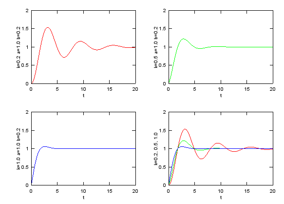
A smaller k gives a larger first peak and a longer ringing time around the final value of 1.

The exact equation for this form : y = 1 + e^-kt(-a cos t - b sin t) satisfies y'' + 2k y' + (1 + k²) y = 1 + k². So the input F(t) is a constant, and the damping coefficient is 2k. The letter a has two meanings here: the damping coefficient in the equation of the text, and the cosine amplitude in the formula.
The ringing frequency is exactly 1 only in that form : with y'' + c y' + y, the solution rings at sqrt(1 - c²/4) rad/s. The formula keeps the frequency at 1 because its y coefficient is 1 + k².
The first peaks : the peak values are about 1.53 for k = 0.2, 1.22 for k = 0.5 and 1.06 for k = 1.0. They occur near t = 3.1, 2.9 and 2.6.
Only k = 0.2 starts flat : the slope at t = 0 is k a - b. With a = 1.0 and b = 0.2, this is 0 for k = 0.2, 0.3 for k = 0.5 and 0.8 for k = 1.0. A system that starts at rest has zero slope, so only the first curve is an exact step response from rest.
A constant input gives a step response : a forced oscillation in the strict sense has a periodic input F(t). Its solution has this decaying part plus a steady sinusoid at the input frequency.

t=0:0.02:20;
k = 0.2;
a = 1.0;
b = 0.2;
e1 = exp(-k.*t).*(-a.*cos(t)-b.*sin(t)) + 1;
k = 0.5;
a = 1.0;
b = 0.2;
e2 = exp(-k.*t).*(-a.*cos(t)-b.*sin(t)) + 1;
k = 1.0;
a = 1.0;
b = 0.2;
e3 = exp(-k.*t).*(-a.*cos(t)-b.*sin(t)) + 1;

subplot(2,2,1);plot(t,e1,'r-');axis([t(1) t(end) 0 2]);xlabel('t');ylabel('k=0.2 a=1.0 b=0.2');
subplot(2,2,2);plot(t,e2,'g-');axis([t(1) t(end) 0 2]);xlabel('t');ylabel('k=0.5 a=1.0 b=0.2');
subplot(2,2,3);plot(t,e3,'b-');axis([t(1) t(end) 0 2]);xlabel('t');ylabel('k=1.0 a=1.0 b=0.2');
subplot(2,2,4);plot(t,e1,'r-',t,e2,'g-',t,e3,'b-');axis([t(1) t(end) 0 2]);xlabel('t');ylabel('k=0.2, 0.5, 1.0');

Tranfer Function - Tracking without overshoot

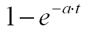
A tracking system has to follow a new target value. The simplest one moves toward the target smoothly and never passes it. Its response to a step input of 1 is 1 - e^-at.

This form is presentation for the simplest and most fundamental part of control system transfer function. (This is often called '1st order delay function'

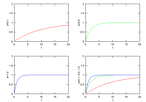
First order step responses for a equal to 0.1, 0.5 and 1.0

A larger a reaches the target faster, and no curve ever goes above 1.

The transfer function is a/(s + a) : its step response is 1 - e^-at. It has one pole at s = -a on the negative real axis, so the response has no oscillation.
1/a is the time constant : at t = 1/a the output reaches 1 - e^-1, about 63.2% of the target. It reaches about 99.3% at t = 5/a.
Reading the plots : a = 0.1 has a time constant of 10, so it is still at about 86% at t = 20. The curves for a = 0.5 and a = 1.0 have time constants of 2 and 1, so they reach the target well before t = 20.
The slope is largest at t = 0 : the curve starts rising at once with slope a, and the slope only decreases after that. The second order forms in the next sections behave differently at the start.

t=0:0.02:20;
a = 0.1;
e1 = 1-exp(-a.*t);
a = 0.5;
e2 = 1-exp(-a.*t);
a = 1.0;
e3 = 1-exp(-a.*t);

subplot(2,2,1);plot(t,e1,'r-');axis([0 20 0 2]);xlabel('t');ylabel('a=0.1');
subplot(2,2,2);plot(t,e2,'g-');axis([0 20 0 2]);xlabel('t');ylabel('a=0.5');
subplot(2,2,3);plot(t,e3,'b-');axis([0 20 0 2]);xlabel('t');ylabel('a=1.0');
subplot(2,2,4);plot(t,e1,'r-',t,e2,'g-',t,e3,'b-');axis([0 20 0 2]);xlabel('t');ylabel('a=0.1, 0.5, 1.0');

Transfer Function - Tracking with overshoot/without oscillation

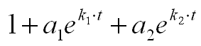
This example shows the following representation. The graph for this function is shown in thick black curve in the last graph, but it would not be easy to understand how the combination of a couple of exponential function can create such a graph. So I plotted the three component (1, a1 exp(k1 t), a2 exp(k2 t)) separately. This is also very important form of graph in Control System designa and analysis. (This form is often called '2nd order delay function').

Examine the sign of each values (a1, a2, k1, k2) in the following example. You would have totally different shape of curve depending on the sign of these values.

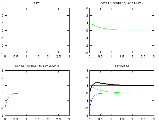
Formula 1 plus a1 e to the power k1 t plus a2 e to the power k2 t

The three components and their sum for a1 equal to 1, k1 equal to -2, a2 equal to -2 and k2 equal to -8

The fast negative term cancels the other two terms at t = 0. The slow positive term then creates the overshoot before the sum settles at 1.

The sum starts at 0 : at t = 0 the sum is 1 + a₁ + a₂ = 1 + 1 - 2 = 0.
The overshoot is 37.5% : the peak is where the slope -2e^-2t + 16e^-8t is 0, that is at t = ln 8/6, about 0.347. The value there is 1 + 0.5 - 2 x 0.0625 = 1.375.
Two real poles alone do not overshoot : this curve is the step response of (14s + 16)/((s + 2)(s + 8)). The poles at -2 and -8 are real, so there is no oscillation. The overshoot comes from the zero at s = -16/14, about -1.14. Without the zero, the transfer function is 16/((s + 2)(s + 8)). Its step response, 1 - (4/3)e^-2t + (1/3)e^-8t, never goes above 1.
The initial slope shows the zero : the slope at t = 0 is a₁k₁ + a₂k₂ = -2 + 16 = 14. A system with two poles and no zero starts with zero slope.

% 1 + a1 e^(k1 t) + a2 e^(k2 t)
t=0:0.02:3;
a1=1;
a2=-2;
k1=-2;
k2=-8;
e1 = 0 .* t .+ 1;
e2 = a1 .* exp(k1 .* t);
e3 = a2 .* exp(k2 .* t);
e4 = e1 + e2 + e3;

subplot(2,2,1);plot(t,e1,'r-');axis([0 3 -3 3]);xlabel('t');title('e1=1');
subplot(2,2,2);plot(t,e2,'g-');axis([0 3 -3 3]);xlabel('t');title('e2=a1 * exp(k1 * t), a1=1,k1=-2');
subplot(2,2,3);plot(t,e3,'b-');axis([0 3 -3 3]);xlabel('t');title('e3=a2 * exp(k2 * t), a2=-2,k2=-8');
subplot(2,2,4);plot(t,e1,'r-',t,e2,'g-',t,e3,'b-',t,e4,'k-','linewidth',3);axis([0 3 -3 3]);xlabel('t');title('e1+e2+e3');

Transfer Function - Tracking with overshoot/with oscillation

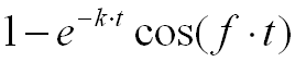
When the two poles are complex, the response oscillates as well as overshoots. The form 1 - e^-kt cos(ft) is the simplest way to write it. Here k sets how fast the oscillation decays, and f sets how fast it oscillates.

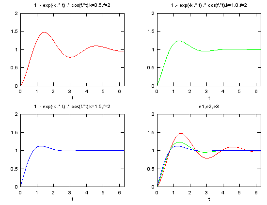
Formula 1 minus e to the power minus k t times cos of f t

Damped oscillating step responses for k equal to 0.5, 1.0 and 1.5 with f equal to 2

A larger k damps the oscillation faster and lowers the first peak, while f = 2 keeps the same timing.

The poles are at -k +/- jf : the transfer function behind this step response is (ks + k² + f²)/((s + k)² + f²). The real part -k gives the decay, and the imaginary part f gives the oscillation. This is the spiral of the earlier sections, seen through its real part.
The first peaks : the peak is about 1.47 at t = 1.45 for k = 0.5, 1.23 at t = 1.34 for k = 1.0 and 1.12 at t = 1.25 for k = 1.5.
The period is 2π/f : with f = 2 this is π, about 3.14. So the k = 0.5 curve has its first minimum near t = 3.0 and its second peak near t = 4.6.
The initial slope is k, not 0 : so this form also contains a zero, as in the previous section. The standard second order step response adds a sine term, 1 - e^-kt(cos ft + (k/f) sin ft), and it starts with zero slope.

% 1 - e^(-k t) cos(f t)
t=linspace(0,2*pi,100);
k=0.5;
f=2;
e1 = 1 .- exp(-k .* t) .* cos(f.*t);

k=1.0;
f=2;
e2 = 1 .- exp(-k .* t) .* cos(f.*t);

k=1.5;
f=2;
e3 = 1 .- exp(-k .* t) .* cos(f.*t);

subplot(2,2,1);plot(t,e1,'r-');axis([t(1) t(end) 0 2]);xlabel('t');title('1 .- exp(-k .* t) .* cos(f.*t),k=0.5,f=2');
subplot(2,2,2);plot(t,e2,'g-');axis([t(1) t(end) 0 2]);xlabel('t');title('1 .- exp(-k .* t) .* cos(f.*t),k=1.0,f=2');
subplot(2,2,3);plot(t,e3,'b-');axis([t(1) t(end) 0 2]);xlabel('t');title('1 .- exp(-k .* t) .* cos(f.*t),k=1.5,f=2');
subplot(2,2,4);plot(t,e1,'r-',t,e2,'g-',t,e3,'b-');axis([t(1) t(end) 0 2]);xlabel('t');title('e1,e2,e3');