In this page, I will describe how to represent various spring systems using stiffness matrix. However, I will not explain much of underlying physics to derive the stiffness matrix. I would describe more about how to construct the matrix from simple building block matrix. You can derive the same matrix based on physics as described in FEM(Finite Element Method) - Simple Spring Model and FEM(Finite Element Method) - More Complicated Spring Model. I would recommend you to go through these page and have some understandings on physics background first if you don't extremly hate physics :).  

However, if the system gets more complicated (i.e, more springs gets connected) it would be difficult to derive the matrix purely based on physics. You will notice how convinient it is to construct the matrix in the page described here.

The whole page follows one recipe. Each spring gives a small building block matrix. The blocks are added into one large matrix by node number, and the rows and columns of fixed nodes are removed at the end. The first five sections apply the recipe to springs on a line, where each node moves in one direction only. The next two repeat it on a 2D plane, where each node moves in x and in y. The last section shows how to check the assembled matrix and solve it for the displacements.

• Single Spring - Free Ends
• Single Spring - A Fixed End
• Double Spring - Free Ends
• Double Spring - A Fixed End
• Complicated Spring System I
• Single Spring on 2D plane
• Double Spring on 2D plane
• How do you check and solve an assembled stiffness matrix ?

Single Spring - Free Ends

Most of the stiffness matrix starts with the following building block. This is for a system made up of the single spring and both ends of the spring can move freely in horizontal direction. The stiffness matrix and the equation for hook's law is as follows.  The stiffness matrix for any spring system, however complex it is, can be construced by combining these building blocks.

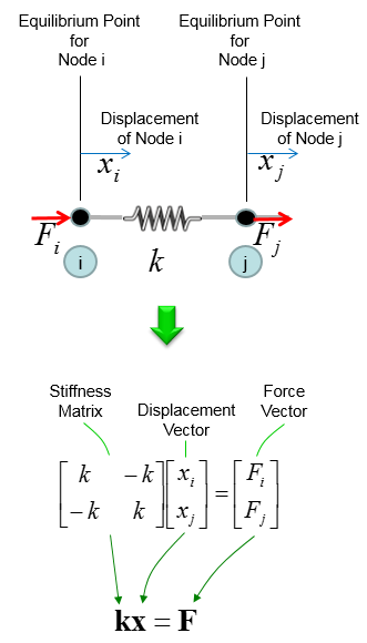
Figure 1. Single spring with two free ends. The 2 x 2 matrix links the two node displacements to the two node forces, and every larger system on this page is built from copies of it.

• The top half is the physical model : node i and node j sit at the two ends of spring k. Each node has its own displacement, x_i or x_j, measured from its equilibrium point, and its own force, F_i or F_j.
• The bottom half is the matrix form : the stiffness matrix times the displacement vector gives the force vector. The whole equation is written in short as kx = F.

Let's read the two rows of the matrix. The first row says F_i = k x_i - k x_j = k(x_i - x_j). The second row says F_j = k(x_j - x_i). So the spring responds only to the difference of the two displacements, which is its stretch. The two forces are always equal and opposite, because F_i + F_j = 0.

This has one consequence for the rest of the page. If both nodes move by the same amount, the stretch is zero and both forces are zero. This is a rigid-body motion, and the matrix cannot tell it apart from no motion at all. In matrix terms, the determinant is k² - (-k)(-k) = 0, and the rank is 1. So you cannot invert this matrix to get the displacements from the forces. At least one node has to be fixed first, and the next section does exactly that.

• Each row of the matrix sums to zero : k + (-k) = 0. This holds for every free-ends stiffness matrix on this page, and it is a quick check after assembly.
• The matrix is symmetric : the entry in row i, column j equals the entry in row j, column i. Adding blocks together keeps this property.
• A free-ends matrix is singular : a system that can slide as a whole has no unique displacement for a given force.

Single Spring - A Fixed End

Another important building block is shown below. It is also a single spring system but in this case one end of the spring is fixed.  Basically the stiffness matrix for this system can be derived from the case of free ends (shown in previous section).  Fixed end means that the displacement of that end is always zero. The derivation of stiffness matrix for this case is based on this fact (i.e, displacement = 0 at the fixed end).

Overall procedure to derive the stiffness matrix is shown below.

At Step (A) : Illustrate the system

At Step (B) : Construct stiffness matrix and Hook's formula as if there is no fixed end (i.e, assume all ends are free).

At Step (C) : You can take two different procedure at this point.

Case (1) Remove the columns and rows that is associated with fixed node (fixed end). In this case, node (i) is fixed. So column (i) and row (i) is removed and we will get the resulting equation as (1). In this case, the size (dimension) of the matrix decreases. This is the most typical way that are described in most of the text book.

Case (2) Replace the columns and rows that is associated with fixed node (fixed end) with zero. Then you will get the equation as in (2). In this case, the size of the matrix does not change as in free end case. This is not usually introduced in any textbook, but I am introducing this case since it would be easier to contruct the matrix if you implement the system with software program.

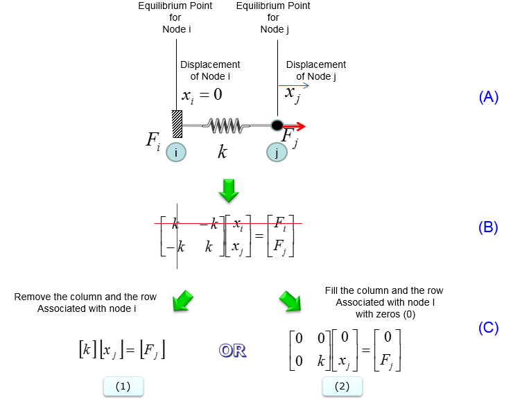
Figure 2. Single spring with node i fixed. Removing the row and column of node i gives the 1 x 1 equation k x_j = F_j. Filling them with zeros keeps the 2 x 2 size.

• Step (A) : node i is attached to a wall, so x_i = 0. The force F_i is now the reaction force from the wall.
• Step (B) : the red lines cross out the row and the column of node i in the free-ends matrix.
• Step (C), equation (1) : only k x_j = F_j remains. This is Hooke's law for a spring with one end on a wall.
• Step (C), equation (2) : the matrix stays 2 x 2, with zeros in the row and the column of node i.

Why is it allowed to cross out the column of node i ? Column i multiplies x_i, and x_i = 0, so that column adds nothing to any force. The row of node i is different. It holds the unknown reaction force F_i, not a given load. So it is taken out of the set of equations to solve. After you find x_j, you can still get the reaction force from the removed row: F_i = -k x_j.

Be careful with Case (2) when you pass the matrix to a numerical solver. The zero row and the zero column make the matrix singular, because its determinant is 0. A common software fix is to put 1 on the diagonal of the fixed node and 0 in its force entry. The equation for that node then reads x_i = 0, and the matrix becomes invertible without changing its size.

• A fixed node removes one unknown displacement : its displacement is known to be zero, so its column carries nothing.
• The removed row still gives the reaction force : evaluate it after you solve for the free displacements.
• Case (1) and Case (2) give the same displacements : Case (2) only needs the diagonal fix before a solver can invert it.

Double Spring - Free Ends

Now let's see a little bit more complicated system and see how the building blocks shown above are used to represent more complicated system. The new question here is what happens at a node that two springs share.

In this system, you have two springs connected together as shown below.

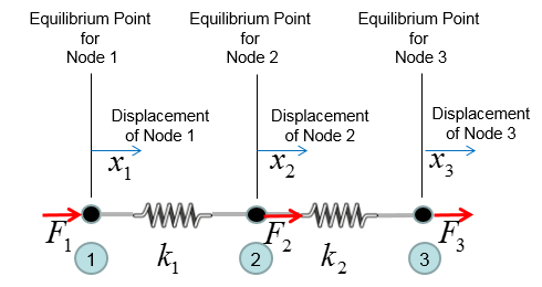
Figure 3. Two springs in series with three free nodes. Node 2 is shared by spring k₁ and spring k₂.

Now you can divide this system into two building block as shown below. However complex system it is, you can always breakdown the system into multiple building blocks.

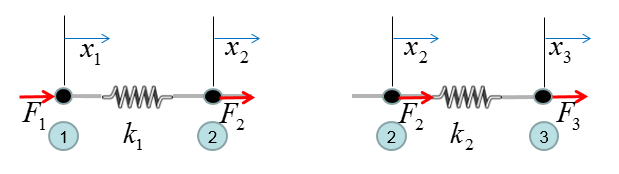
Figure 4. The same system split into two single-spring building blocks. Node 2 appears in both blocks.

Now from this building block, you can construct the stiffness matrix and Hook's equation as follows.

Step (A) : Breakdown the system into building blocks

Step (B) : Construct the stiffness matrix and Hook's equation for each building block. And label each column and raw with the number of each node. Dimension of each matrix will be always 2 x 2. If you get familiar with this process, you may skip this step and go directly to Step (C).

Step (C) : Create a big stiffness matrix and Hooks equation that can accommodate the whol system. The size of the matrix became N by N, where N indicates the total number of nodes in the system. Since the number of the nodes in this example is 3, the size (dimension) of the matrix become 3 x 3. Then, plug the matrix of the building blocks into the large matrix according to the index number.

Step (D) : Superimpose all the matrix equation from Step (C) into single system matrix. In this process, just do matrix sum of stiffness matrix.  Do vector sum of displacement vector. But you should be careful with combining Force vector. As you see in the result, the force vector F is a little bit different from vector sum of each building block.  If you do vector sum of F vector, it would become [F1, 2 F2, F3]. However, you have to divide (2 F2) by 2, because the node (node 2 in this case) is used twice.

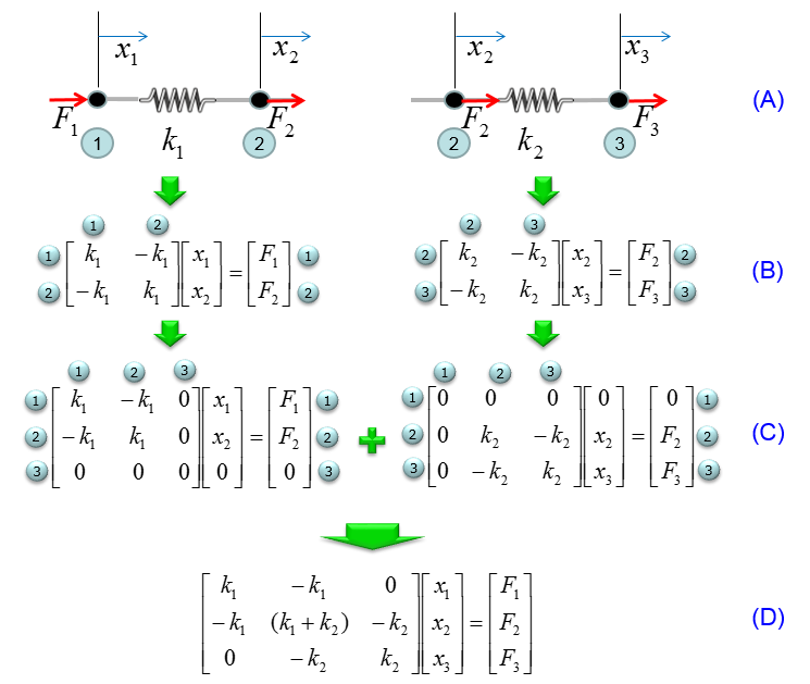
Figure 5. Assembly of the two blocks. Each 2 x 2 block is placed into a 3 x 3 matrix by node number, and the two 3 x 3 matrices are added.

• Step (A) : the two building blocks, each with its own pair of nodes.
• Step (B) : the 2 x 2 matrix of each block. The circled numbers label each row and column with its node.
• Step (C) : each block expanded to 3 x 3. The rows and columns of the node that a block does not touch are zero.
• Step (D) : the sum. The shared node 2 collects k₁ + k₂ on its diagonal.

Let's look again at the force vector in Step (D). Each block has its own F₂, but the two are not the same force. The F₂ of the left block is the part of the node 2 force that spring k₁ carries. The F₂ of the right block is the part that spring k₂ carries. The external force on node 2 is the sum of these two parts. So the assembled vector [F₁, F₂, F₃] is correct when F₂ means the total force on node 2. The division by 2 in Step (D) only undoes the use of the same symbol F₂ for two different parts.

The displacement vector is not added at all. Both blocks use the same x₂, because one node can be in only one place. So the assembled vector is simply [x₁, x₂, x₃], as Step (D) shows. You can confirm the middle row with physics too. It reads F₂ = k₁(x₂ - x₁) + k₂(x₂ - x₃), which is the pull of both springs on node 2.

• Assembly adds matrices, it never multiplies them : each spring adds its own entries into the rows and columns of its two nodes.
• A diagonal entry is the sum of the springs attached to that node : node 2 touches k₁ and k₂, so its diagonal entry is k₁ + k₂.
• An off-diagonal entry is minus the spring between two nodes : row 1, column 3 is 0, because no spring connects node 1 and node 3.
• The 3 x 3 result is still singular : each row still sums to zero, and the rank is 2. The chain as a whole can still slide.

Double Spring - A Fixed End

Now let's look at a variation of two spring system. As you see in the following illustration, it is almost same as previous example. The only difference is that node 1 is fixed in this example.

So the overal procedure for matrix construction is very similar to previous example.

Step (A) : Illustrate the system

Step (B) : Construct the stiffness matrix and Hook's equation for the case where there is no fixed node.

Step (C) : You can take two different procedure at this point.

Case (1) Remove the columns and rows that is associated with fixed node (fixed end). In this case, node 1 is fixed. So column 1 and row 1 is removed and we will get the resulting equation as (1). In this case, the size (dimension) of the matrix decreases. This is the most typical way that are described in most of the text book.

Case (2) Replace the columns and rows that is associated with fixed node (fixed end) with zero. Then you will get the equation as in (2). In this case, the size of the matrix does not change as in free end case. This is not usually introduced in any textbook, but I am introducing this case since it would be easier to contruct the matrix if you implement the system with software program.

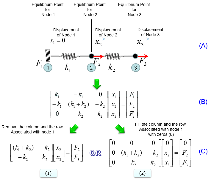
Figure 6. Two springs with node 1 fixed. Removing row 1 and column 1 leaves a 2 x 2 matrix for the free nodes 2 and 3.

• Step (A) : node 1 is on the wall, so x₁ = 0.
• Step (B) : the free-ends 3 x 3 matrix from the previous section, with row 1 and column 1 crossed out.
• Step (C), equation (1) : the reduced 2 x 2 equation for x₂ and x₃.
• Step (C), equation (2) : the 3 x 3 form with zeros in row 1 and column 1.

Let's solve equation (1) with numbers. Take k₁ = 100 N/m and k₂ = 200 N/m, with F₂ = 0 and F₃ = 10 N. The reduced matrix is [300, -200; -200, 200], and its determinant is 300 x 200 - 200 x 200 = 20000. The solution is x₂ = 0.1 m and x₃ = 0.15 m.

You can check this result with plain physics. The 10 N load passes through both springs in series. Spring k₁ stretches by 10/100 = 0.1 m, and spring k₂ stretches by 10/200 = 0.05 m. So node 3 moves 0.1 + 0.05 = 0.15 m. The removed row 1 gives the wall reaction F₁ = -k₁x₂ = -10 N, which balances the load.

• Fixing one node makes the matrix invertible : the determinant of the reduced matrix is k₁k₂, which is nonzero whenever both springs have stiffness.
• The fixed node can be any node : fixing node 3 instead would remove row 3 and column 3. The procedure is the same.
• A physics check catches assembly errors : a series chain must stretch by F/k₁ + F/k₂ at its free end.

Complicated Spring System I

Now I will show you another example which is much more complicated shown below. I have shown you the exact same case in FEM(Finite Element Method) - More Complicated Spring Model. But the way to construct the stiffness matrix will be a little bit different here. Personally I prefer the procedure that I will show you in this page. It will take a little bit more steps but you will be able to create the stiffness matrix without much thinking or confusion if you use the method being used in this page.

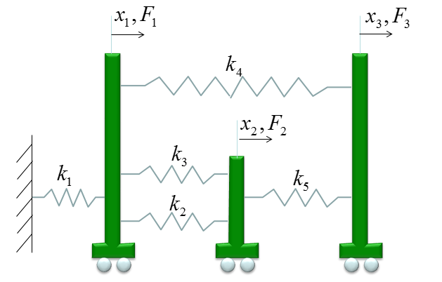
Figure 7. The original system. Three carts on rollers are connected by five springs, and spring k₁ ties cart 1 to a wall.

As a first step, I changed the system a little as shown below. This is to convert the fixed node to free node. and I will derive the stiffness matrix and Hook's equation for this all free-end system first. And I assigned the number Zero to the freed node. The reason why I put the number 0 is to keep the same number for all the other nodes as in the original.

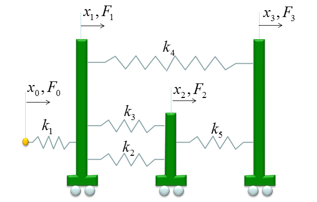
Figure 8. The wall is replaced by a free node 0. The whole system is first treated with free ends, and node 0 is fixed at the end.

First, you need to figure out the size of the stiffness matrix for the whole system. Do you know what it is ?

It is 4x4 because you have four nodes (0,1,2,3) in this example.  With this in mind, let's go through matrix construction.

First, constuct fill in the matrix with stiffness values for the spring k1 which is connecting the node 0 and node 1. It become as follows.

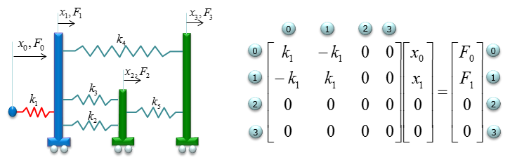
Figure 9. Contribution of spring k₁, between node 0 and node 1. Only rows and columns 0 and 1 are nonzero.

Next, constuct fill in the matrix with stiffness values for the spring k2 which is connecting the node 1 and node 2. It become as follows.

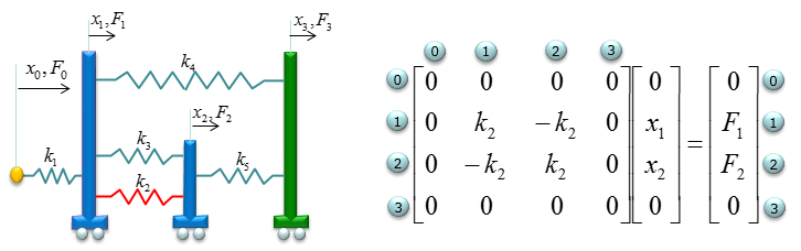
Figure 10. Contribution of spring k₂, between node 1 and node 2.

Next, constuct fill in the matrix with stiffness values for the spring k3 which is also connecting the node 1 and node 2. It become as follows.

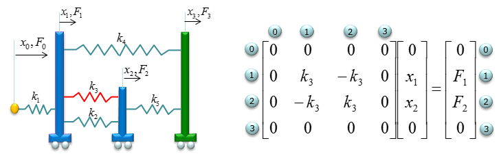
Figure 11. Contribution of spring k₃. It connects the same two nodes as k₂, so it fills the same four entries.

Next, constuct fill in the matrix with stiffness values for the spring k4 which is also connecting the node 1 and node 3. It become as follows.

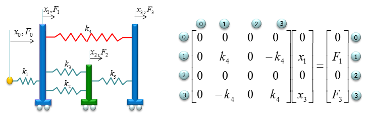
Figure 12. Contribution of spring k₄, between node 1 and node 3. It puts k₄ on the diagonal of node 1 and of node 3.

Last, constuct fill in the matrix with stiffness values for the spring k5 which is also connecting the node 2 and node 3. It become as follows.

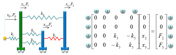
Figure 13. Contribution of spring k₅, between node 2 and node 3.

Now combining (superimposing) all of the matrix, you will get a matrix equation as follows.

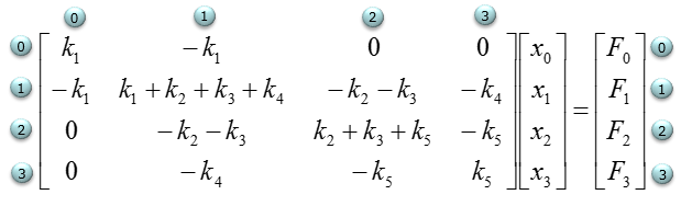
Figure 14. Sum of the five contributions for the all free-ends system. The entry in row 3, column 3 should read k₄ + k₅, as explained below.

The above matrix is for the system without any fixed node. But the original problem is to construct matrix for the node 0 fixed. So we need to convert this all free-ends system matrix into the one with node 0 fixed.  As you learned from the examples above, it is very simple as shown below.

Case (1) Remove the columns and rows that is associated with fixed node (fixed end). In this case, node 0 is fixed. So column 0 and row 0 is removed and we will get the resulting equation as (1). In this case, the size (dimension) of the matrix decreases. This is the most typical way that are described in most of the text book.

Case (2) Replace the columns and rows that is associated with fixed node (fixed end) with zero. Then you will get the equation as in (2). In this case, the size of the matrix does not change as in free end case. This is not usually introduced in any textbook, but I am introducing this case since it would be easier to contruct the matrix if you implement the system with software program.

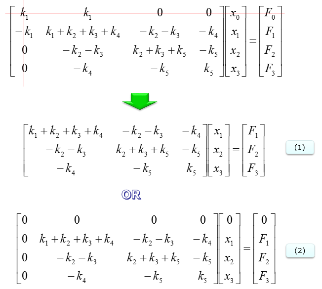
Figure 15. Node 0 fixed. Removing row 0 and column 0 gives the 3 x 3 equation (1), and zero filling them gives the 4 x 4 equation (2).

• Top : the free-ends matrix of Figure 14, with row 0 and column 0 crossed out.
• Equation (1) : the reduced 3 x 3 system for x₁, x₂ and x₃.
• Equation (2) : the 4 x 4 form with zeros in row 0 and column 0.

Before you use the assembled matrix, check it against the rules from the double spring section. Node 3 has two springs attached, k₄ and k₅. So its diagonal entry must be k₄ + k₅, and the k₄ contribution in Figure 12 does put k₄ there. Figure 14, however, shows only k₅ in row 3, column 3. The row-sum test finds the same error, because row 3 sums to -k₄ - k₅ + k₅ = -k₄ instead of 0. Equations (1) and (2) in Figure 15 carry the same entry, so read it as k₄ + k₅ there too. The crossed-out row 0 of Figure 15 also shows k₁ in column 1 where it should be -k₁. That row is removed, so this slip does not change the result.

With that correction, the reduced matrix for node 0 fixed is shown in the table below. Every diagonal entry is the sum of the springs at that node, not counting k₁ at nodes other than node 1.

Let's put numbers in. Take k₁ to k₅ = 100, 200, 300, 400 and 500 N/m, and a single load F₃ = 10 N on cart 3. The solution is x₁ = 0.1 m, x₂ = 0.1077 m and x₃ = 0.1154 m. The value of x₁ is easy to check. The whole 10 N load has to reach the wall through k₁, so cart 1 moves 10/100 = 0.1 m. If you solve with the k₅-only entry of Figure 14 instead, you get negative displacements of about -0.03 m. A pull to the right cannot move every cart to the left, so the error shows up at once.

• Build the free-ends matrix first, then fix nodes : adding a dummy node 0 for the wall keeps every spring in the same 2 x 2 form.
• One spring touches exactly four entries : the two diagonal entries of its nodes and the two entries that connect them.
• Parallel springs simply add : k₂ and k₃ join the same two nodes, so they act as one spring of stiffness k₂ + k₃.
• Row sums and symmetry catch most slips : run both checks on the free-ends matrix before you remove any row.

Single Spring on 2D plane

So far every node could move along one line only. On a plane, each node can move in x and in y, so each node carries two displacements and two forces. The spring itself still reacts only to the change of its length along its own axis. This section projects that 1D spring onto the x and y axes, and the result is a 4 x 4 matrix instead of a 2 x 2 one.

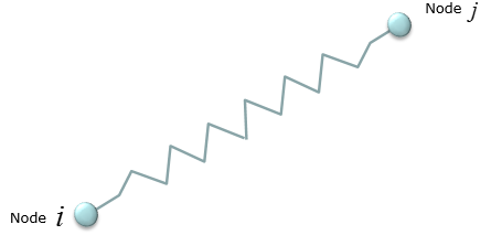
Figure 16. A spring between node i and node j, placed at an angle on the plane.

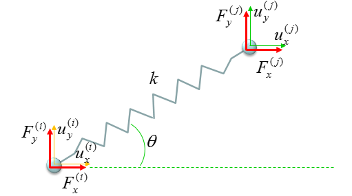
Figure 17. Displacements u and forces F at each node, split into x and y components. The angle θ is measured from the x axis to the spring.

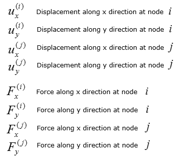
Figure 18. Symbols of the 2D element. Each node has two displacements and two forces.

The matrix below is built from Figure 17 and the symbols in Figure 18. Note that its labels use the superscripts (1) and (2) for node i and node j.

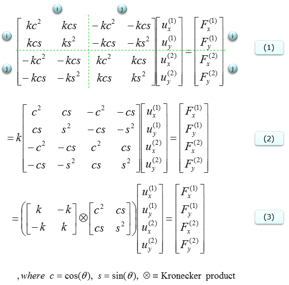
Figure 19. The 4 x 4 element stiffness matrix of a 2D spring in three equal forms. Form (3) writes it as the 1D spring matrix Kronecker-multiplied by a 2 x 2 direction block.

• Form (1) : the four rows split into two node blocks, i and j. Each block is 2 x 2 because each node has an x row and a y row.
• Form (2) : the same matrix with the common factor k taken out, where c = cos θ and s = sin θ.
• Form (3) : the 1D matrix [k, -k; -k, k] Kronecker-multiplied by [c², cs; cs, s²]. Each entry of the 1D matrix is replaced by that entry times the direction block.

Where do c², cs and s² come from ? The spring stretches only by the part of the relative displacement that lies along its axis. The unit vector along the spring is (c, s). So the stretch is c(u_x^(j) - u_x⁽ⁱ⁾) + s(u_y^(j) - u_y⁽ⁱ⁾). The spring force is k times this stretch, and it acts along the same axis. Its x and y components are that force times c and times s. Multiplying the two projections gives c², cs and s² in every 2 x 2 block.

Two special angles make a good check. At θ = 0, c = 1 and s = 0, so only the x rows remain, and they hold the 1D matrix from the first section. At θ = 90 deg, only the y rows remain. For a spring from (0, 0) to (3, 4), c = 0.6 and s = 0.8, so the direction block is [0.36, 0.48; 0.48, 0.64]. Expanding the Kronecker product with this block reproduces form (2) entry by entry.

In a program, you rarely know the angle θ directly. You usually know the coordinates of the two nodes, and c and s follow from them.

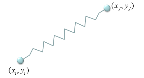
Figure 20. The node coordinates, which give the direction of the spring.

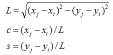
Figure 21. Length L and direction cosines c and s from the node coordinates. The sign inside the square root should be +, as explained below.

The length formula in Figure 21 has a minus sign between the two squares. The correct formula is the distance between the two nodes, L = √((x_j - x_i)² + (y_j - y_i)²). With the minus sign, the 3-4 example above would give √(9 - 16), which is not a real number. The formulas for c and s are correct, and they satisfy c² + s² = 1.

• Each node owns two rows and two columns : a 2D spring element is 4 x 4, and a system of N nodes gives a 2N x 2N matrix.
• The 2D matrix is still singular : its rank is 1, and its eigenvalues are 0, 0, 0 and 2k. The three zero modes are the two translations and a small rotation, which do not stretch the spring.
• The direction block carries all the geometry : the stiffness k and the node numbering work exactly as in the 1D case.

Double Spring on 2D plane

Two springs on a plane follow the same recipe as two springs on a line. Only the block size changes. Each node now owns two rows and two columns, so a system of three nodes gives a 6 x 6 matrix instead of a 3 x 3 one. Each spring also has its own angle, so each one has its own c and s.

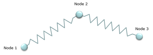
Figure 22. Three nodes on a plane connected by two springs. Node 2 is the shared node.

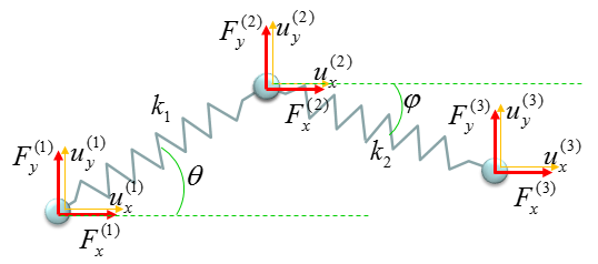
Figure 23. Displacement and force components at each node. Spring k₁ rises at angle θ, and spring k₂ falls at angle φ below the horizontal.

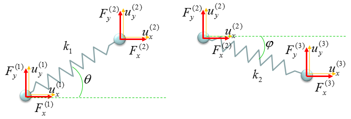
Figure 24. The system split into two 2D building blocks.

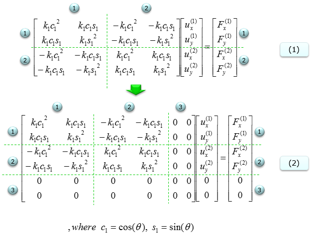
Figure 25. Block of spring k₁. Its 4 x 4 matrix is expanded to 6 x 6, with zeros in the rows and columns of node 3.

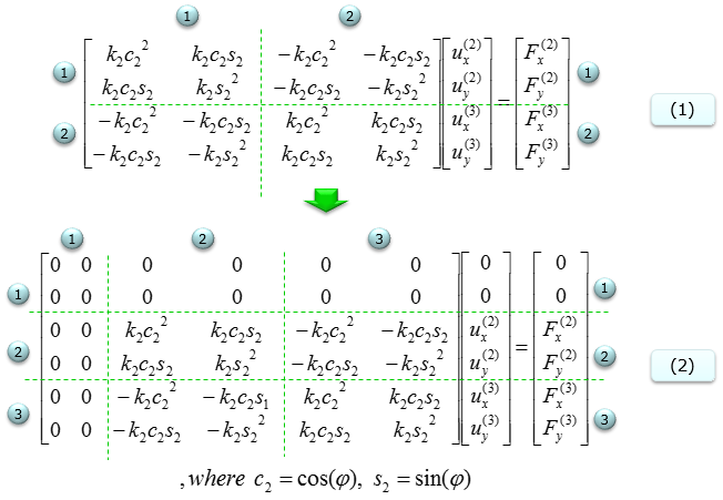
Figure 26. Block of spring k₂. Its 4 x 4 matrix is expanded to 6 x 6, with zeros in the rows and columns of node 1.

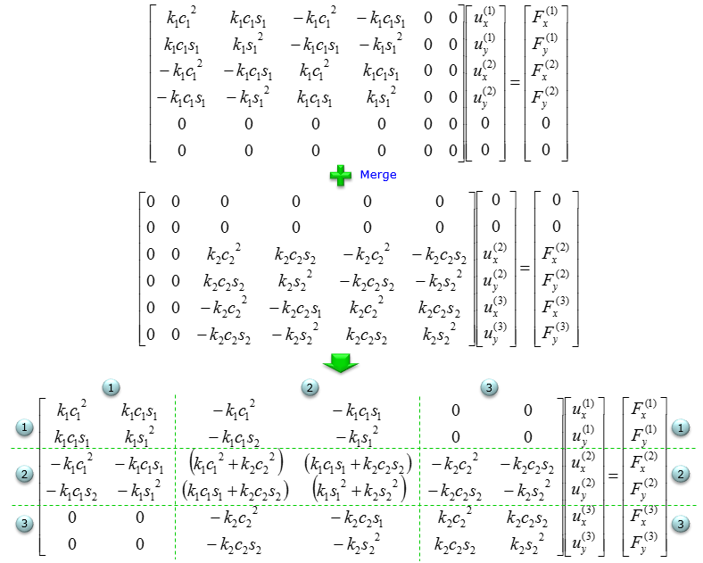
Figure 27. Sum of the two 6 x 6 matrices. The 2 x 2 block of the shared node 2 collects terms from both springs.

• Node 1 and node 3 blocks : each holds the terms of one spring only, because each of these nodes touches one spring.
• Node 2 block : k₁c₁² + k₂c₂² and the other sums on the diagonal come from both springs.
• Blocks between node 1 and node 3 : they are zero, because no spring connects the two nodes.

Figure 26 and Figure 27 contain a few index slips. Every product in the k₁ terms uses c₁ and s₁, and every product in the k₂ terms uses c₂ and s₂. So the entries shown as -k₂c₂s₁ should read -k₂c₂s₂. In the assembled matrix of Figure 27, the two entries shown as -k₁c₁s₂ should read -k₁c₁s₁. With these corrections the matrix is symmetric, as every stiffness matrix must be.

Watch the sign of the angle for spring k₂. The formulas in the single spring section measure the angle counterclockwise from the x axis. Spring k₂ falls from node 2 to node 3, so its direction angle is -φ, not φ. This gives c₂ = cos φ but s₂ = -sin φ. The c₂² and s₂² terms do not change. The c₂s₂ terms, however, change sign. Computing c and s from the node coordinates, as in Figure 21, avoids this trap automatically.

• The recipe does not change in 2D : build each element matrix, place it by node number, and add.
• Every scalar entry becomes a 2 x 2 block : a 3-node chain gives a 6 x 6 matrix.
• Use signed angles or coordinates : a spring that points downward needs a negative s.

How do you check and solve an assembled stiffness matrix ?

Assembly is mechanical, so most mistakes are copying slips, like the node 3 entry in the complicated spring system. Before you solve anything, it pays to run a few checks that need no physics at all. Then the solve itself is one call in any numerical tool. Let's list the checks first and then the solving steps.

The checks in the table below apply to every 1D and 2D stiffness matrix on this page. The examples come from the sections above.

The eigenvalues in the last row use the numbers of the five spring example, k₁ to k₅ = 100 to 500 N/m. A negative or zero eigenvalue after fixing means that a node is still free to drift, or that an entry is wrong.

Once the checks pass, the solve takes four steps. First, assemble the full free-ends matrix K and the force vector F. Second, remove the rows and columns of the fixed nodes, or zero-fill them and put 1 on their diagonal. Third, solve Kx = F for the free displacements with a linear solver, such as x = K\F in Matlab or numpy.linalg.solve(K, F) in Python. A solver is faster and more accurate than forming K^-1 explicitly. Fourth, multiply the removed rows by the solved displacements to get the reaction forces at the fixed nodes.

• Check before you solve : symmetry and row sums take seconds and catch most assembly slips.
• Block all rigid motion : a 1D system needs one fixed node, and a 2D system needs enough supports to stop two translations and one rotation.
• Check the answer with physics : a force that runs through a single spring to the wall must give F/k at that spring, as with x₁ = 0.1 m in the five spring example.
• Use a solver, not the inverse : the solver works directly on K and F, which is how larger FEM programs handle thousands of nodes.