|
Engineering Math |
||
|
Matrix
Matrix would be one of the most important and widely used mathematical tool in engineering. I personally think that you would adapt to almost any engineering field if you are familiar with Differential Equation and Matrix. Personally Matrix is one of the intriguing concept and tools to me. I know many of you would not agree with me especially if you are already got sick and tired of so manycalculations and struggling with Linear Algebra course.
How we use Matrix to solve a real life problem
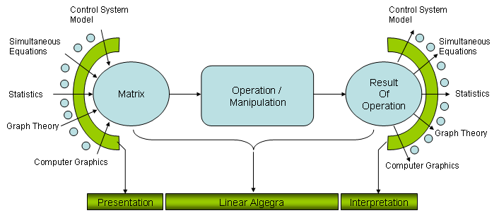
My understanding of use model for Matrix in engineering field is as shown in the following illustration. Try to interpret the illustration from left to right.
i) First, represent your problem in real life into a Matrix form (You will see a couple of examples of these represetations from following sections). ii) And then you would apply various mathematical operations to the Matrix and get the outcome of the operation. (Determining what kind of operatioin you should perform and understand why you should apply those operations should be the critical part at this step). iii) Finally you have to interpret the result of step ii) into your real life situation.
I think one of the biggest reason why your linear algebra course does not interest you (even scarying you away) is that it focus mostly in step ii) and in many case you would not feel such a strong interest to anything which does not show any close relationships to real life problems.
In this page, I would provide you some examples to trying to show you the step i) and step iii) as much as possible and I will keep adding those examples. Of course, only a couple of examples explained here would not be enough to give you strong motivation and understandings on Matrix. But I hope it can at least be a small trigger.
Before I put my own words, I would like to strongly recommend you to see an excellent lecture by Proffer Stephen Boyd. Introduction to Linear Dynamical System. If you want to see the full course, visit here. Interestingly, this lecture shows exactly the approach that I want to take when I am studying Matrix.
< Example 1 : Simultaneous Equation >
This may be one of the most typical application of Matrix. You may still remember from high school math on how to solve a simultaneous equation. If the number of unknown variable is only 2 or 3 as you saw in the high school math class, it would be easier to solve it in the way you learned in the high school math class. But unfortunately most of real life problem is much more complicated than that. The number of unknown variables would be much more than 2 or 3 and in some cases they may amount to several dozens. In such a case, representing the problem in a matrix format and solve the problem with the technique you would learn in Linear Algebra class would be the best solution.
I don't want to turn this page into a Linear Algebra test book. The purpose of this section is just to show an example of the case for matrix representation.
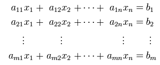
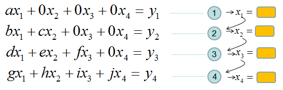
A set of simultaneous equation with n unknown variable can be represented as follows.
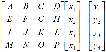
Once you get this kind of simultaneous equation, you can extract coefficient parts, unknown variable and constants parts and can construct a Matrix and two vectors as follows. This is what you already learned from your Linear Algebra course.
Once you got a coefficient matrix and variable vectors, you can represent your original simultaneous equation as follows.
Now a question comes out. Why we need to do this ? After we finish a high school math, all of us would know how to find solutions for a simultaneous equations (I hope you are also a part of this group -:). As far as I remember, I start learning about Simultaneous equation from Junior High and early Senior High. and the learns about using the Matrix to solve a simultaneous equation in the second year in Senior High. At that time, using Matrix for this didn't seem easy to me. Especially finding the solution for the matrix equation using what we called 'Gaussian Elemenation Method' was so complicated to me. And I (also a lot of my friends) said "Why do we have to do this kind of akward things ?". I think the answer to this question is very simple. The common method you learned to solve a simultaneous equation in lower grade of High school would be a good method to find the solution to the simultaneous equation with 2 or 3 variables. Just try to use the same method to solve a simultaneous equation with 10 variables. Then you would realize right away that the method would not be a practical method and you would need something new way to solve it. In addition, most of the real life problem would have much more variables than 10. Some times a single problem would get involved with several hundred variables. In this case, you would realize that Matrix representation is more practical method. A better news is that you only have to convert your problem (a simultaneous equation in this case) into a matrix equation and you don't have to worry about finding solution for it. There are a lot of computer program (e.g, Matlab, Octave, Mathematica and even Microsoft Excel) can find the solution from the Matrix equation. In short, Converting a real life problem into a Matrix format is your job and doing mathemtical operation for solution finding is not your job. It's computer's job.
I have several example that I like for Matrix. Some of the examples, I like them in terms of Modeling which means 'converting a real life problem into a matrix format' and some of the examples, I like them in terms of visualization of the matrix. This example is the one I like in terms of modeling.
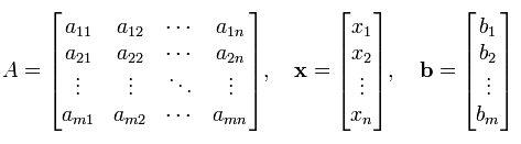
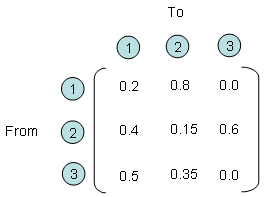
Let's say you have three different entities and all of these three entities interact each other. Every time they interact each other, it gives some portion of what it has to another states and it gets some portioin from other entities. One example with a specific number is as follows. For example, if you look at the entity (2) and entity(1). You would see that these two entities gives something to each other and takes something from each other. More specifically, for every round of interaction, entity (2) gives 40 % of what it has to entity (1) meaning that entity (1) takes 40 % from engity (2) and entity (1) gives 80 % of what is has to entity (2), meaning entity (2) takes 80% from entity (1).
If you describe the relationship between each entity verbally as I described above, you would notice that very soon it gets very complicated and you would forget what you described about entity (1),(2) when you describe entity (2),(1). Furthermore, in most of real life problems the number of entities being involved in the problem tend to be much more than 3. In this case, it is almost impossible to describe all the possible relationships in verbal form. But if you use the matrix form, you can describe this kind of situation in a very simple manner as follows.
Each row number represents the entities where an arrow (shown above) starts and each column represents the entities where an arrow ends. The number within the matrix represents how much amount of things transfers from an entities to another entities. For example, if you see the point where row (2) and colum (3) meets, you see the number '0.6'. It means that for every round of interaction, entity (2) transfer 60 % of what it got to entity (3).
OK.. Now I have a matrix representing how each of entities in a system interact each other. So what ? How can I use this matrix ? I said this matrix represents the interactions among each entities for each round of interaction. What if this kind of interaction repeats 100 times ? If entity (1) had 100, entity (2) has 500 and entity (3) has 300, how much they would get after 100 times of interaction ? Can I get the answers to all of these questions from this matrix ? In conclusion, the answer is YES. and then How ? It is simple, just multiply the same matrix 100 times (Matrix multiplication, not a scalar multiplication) and then you would get the answer for this. Again, you don't have to multiply the matrix 100 times by your hand. Just leave it to the computer. Again, converting a real life problem into a Matrix format is your job and doing mathemtical operation for solution finding is not your job. It's computer's job.
< Example 3 : Neural Network >
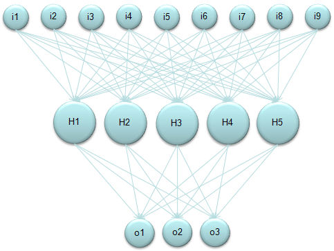
One of the most wildly used form of Neural Network would be illustrated as follows. Here in this diagram,
"i" stands for input layer "H" stands for hidden layer "o" stands for output layer
I am not going to explain what is meaning (role) of these components. Please try google "Neural Network Tutorial" or "Introduction to Neural Network" if you are new to this area.
But the basic calculation logic as as follow. i) Take a Node (a Circle, for example H1). ii) Take all the input value (each arrow) getting into it. iii) Take all the weight value which is associated with each of the input value. iv) Multiply each input value with its corresponding weight value and take the sum of all the multiplication (This is "Sum of Times" process). This become the total input value to the selected Node.
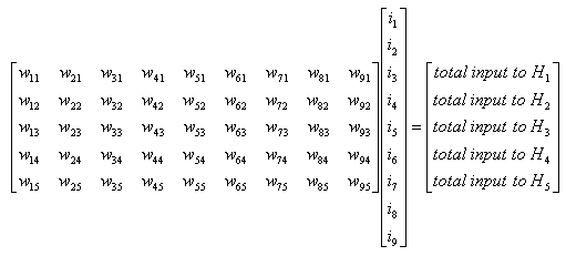
If you do this process for only a single Node (e.g, H1), you can represent it as simple "Sum of Times" form. But if you want to describe this process for all the Nodes at each layer (e.g, H1, H2, H3, H4, H5) it would be easier/clearer to represent it as a Matrix equation as follows. (Of course you can represent this into five separate "Sum of Times/Sum of Multiplication" form, but Matrix form would neat clearer).
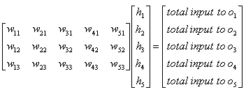
With the same logic as described above, you can get the matrix equation to calculate the total input to the layer 'o (output)'.
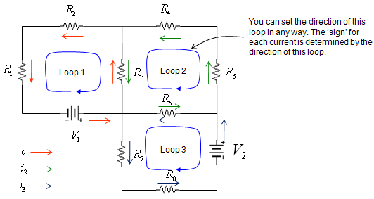
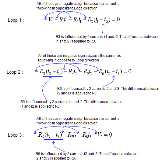
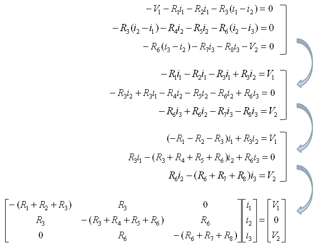
< Example 4 : Circuit Analysis >
< Example 5 : Adjacency Matrix (Graph Theory) >
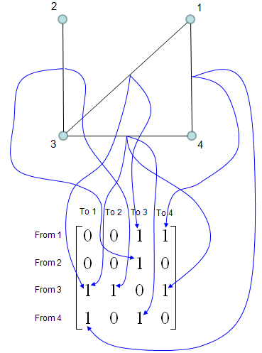
Adjacency Matrix is a matrix which describes the connectivity among the nodes in a graph. (Google "Introduction to Graph Theory" or "Graph Theory Tutorial" if you are new to this area). The way you can construct the Adjacency Matrix from a graph is as follows. I hope this illustrations gives you the intuitive understanding without much description. Basic idea is to put "1" at the matrix element representing two points (from, to) if there is a connection for the two points and put "0" otherwise.
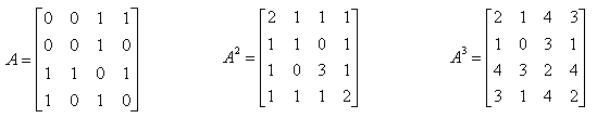
Once you have the Adjacecy Matrix, you can do a lot of mathemtical operation for the matrix to find various useful information. The most common mathematical operation for the Adjacent Matrix is to take "Powers of the matrix". Following shows three matrix, A which is original adjacency Matrix and A^2 and A^3.
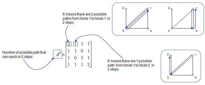
Element value in A^2 is the number of possible paths connecting the two nodes represented by the element. If an element value is "1", it means there is only one path from one node to the other node that is represented by the element. If an element value is "2", it means there are two possible paths from one node to the other node that is represented by the element as illustrated below. In most case, only those elements with the value of "1" has practical meaning.
< Example 6 : FEM(Finite Element Method) - Simple Spring Model >
First I think I should say sorry if you clicked this link in the hope to clear off all the clouds over your head after struggling for so long time trying to understand the details of FEM -:). This is not at all for that level. I just want to give you an idea of application of the mathematical tool called "Matrix" and how a matrix equation is generated from a simple FEM problem. It is true that one of the core part of FEM is converting the problem into a matrix equation, but in reality nobody is doing this by hand because it is too complex to do it manually. There are a lot of software package doing this kind of jobs for various problem spaces. However, understanding this process would be very useful both for understanding the problem space and understanding the logics being used by those software.
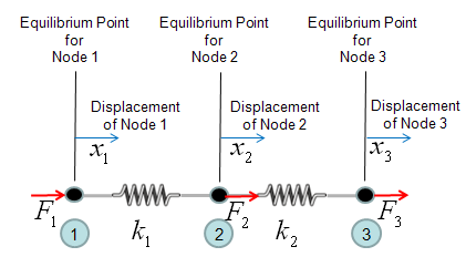
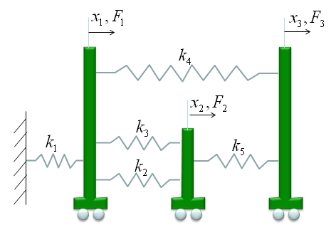
Let's take a very simple cases as follows. You already have seen this problem on many text book or internet pages. Two springs are connected as follows. Let's assume that Node 1 is fixed to a point (like fixed to a wall) and you are pulling away the Node 3. The question how much each of the spring will be elongated ?
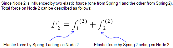
One thing you have to think before you start creating the mathmatical model. It is about node 2. If you see the picture above, node 2 is connected to both spring 1 and spring 2. So it would be experiencing forces from two springs and the force labed as F2 is the total force of the two componend forces. So let's define F2 as follows.
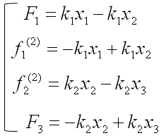
Now by applying the famous hook's law (F = kx), you can draw out four equations as follows.
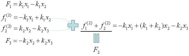
Since the two equation (the second and third one is the force being applied to a single node (Node 2). We can combine the two equeation and as result we would finaly have three equations as follows.
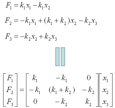
Now we have a set of simultaneous equation comprised of 3 equations. As you already seen above, a simultaneous equation can easily be converted into a matrix equation as follows.
We saw a very simple example of drawing out a matrix equation from a small set of FEM situation, but in real situation.. most of this process is being automatically done by a software. The procedure that the software use to create the final matrix would be a little different from what I described here.. but the resulting matrix equation should be same.
< Example 7 : FEM(Finite Element Method) - More Complicated Spring Model >
In this example, I will introduce a little bit more complicated model than the previous one and I will also show you a new method to construct a Matrix for the system. The method we used in previous example was more relevant to real physical characteristics of the system. But it will be very tedius to construct the matrix via going through every details of physical characteristics. In this example, I will introduce another widely used method but easier to construct a mathematical model. (Note : I got this specific example model from MIT opensource : http://www.youtube.com/watch?v=oNqSzzycRhw and try to describe in my own words).
The model which was given in the lecture linked above is as follows. (You would see this kind of example from various sources with just a little bit of modification, but I intentionally used the model as it is from the above link so that you can learn the same thing from different source (the link above and this page). Of course, the final outcome will be the same but a little bit different way of description)
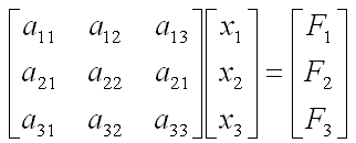
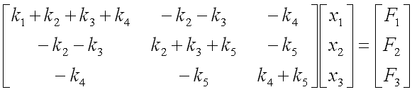
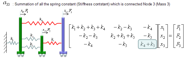
we have three carts connected each other and a fixed point by five springs. This system will be described by the following matrix equation. See the matrix is 3 x 3 matrix and the size of the matrix determined by the number of carts in the model and we call each of the carts as a "Node" in this section. You would notice the size of Matrix is determined by the number of nodes.
Now the question is to determine each of the elements of the matrix according to the condition given in the model. Let me give you the answer key first and let's go through each of the steps to realize the matrix. Just with a brief look, you will notice following characteristics. i) All the values on the diagonal line of the matrix are positive values. ii) All the values not on the diagonal line of the matrix are negative values. iii) Values not on the diagonal line of the matrix are symetric. (e.g, a21 = a12, a31 = a13 etc).
Now let's look into the steps of how we get the values for each of the element.
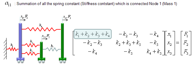
a11 is obtained as shown below. The meaning of a11 is the summation of the spring constants (stiffness constants, k) which are connected to Cart 1 (node 1). As shown below, all the springs connected to Node 1 are shown in red. As you see, spring 1,2,3,4 are connected to node 1. So the value becomes k1+k2+k3+k4.
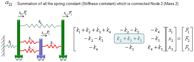
a22 is obtained as shown below. The meaning of a22 is the summation of the spring constants (stiffness constants, k) which are connected to Cart 2 (node 2). As shown below, all the springs connected to Node 2 are shown in red. As you see, spring 2,3,5 are connected to node 2. So the value becomes k2+k3+k5.
a33 is obtained as shown below. The meaning of a33 is the summation of the spring constants (stiffness constants, k) which are connected to Cart 3 (node 3). As shown below, all the springs connected to Node 3 are shown in red. As you see, spring 4,5 are connected to node 3. So the value becomes k4+k5.
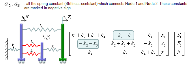
a12 and a21 are obtained as shown below. The meaning of a12 and a21 is the summation of the spring constants (stiffness constants, k) which are connecting Cart 1 and Cart 2 (node 1 and node 2). As shown below, all the springs connecting the two nodes are shown in red. As you see, spring 2,3 are connecting the two nodes. So the value becomes -k2-k3. But notice that these values has negative sign.
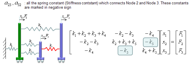
a23 and a32 are obtained as shown below. The meaning of a23 and a32 is the summation of the spring constants (stiffness constants, k) which are connecting Cart 2 and Cart 3 (node 2 and node 3). As shown below, all the springs connecting the two nodes are shown in red. As you see, spring 5 is connecting the two nodes. So the value becomes -k5. But notice that these values has negative sign.
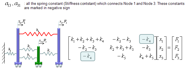
a13 and a31 are obtained as shown below. The meaning of a13 and a31 is the summation of the spring constants (stiffness constants, k) which are connecting Cart 1 and Cart 3 (node 1 and node 3). As shown below, all the springs connecting the two nodes are shown in red. As you see, spring 4 is connecting the two nodes. So the value becomes -k4. But notice that these values has negative sign.
This is more complicated than the previous example, but I hope you might feel easier than the previous one because the steps were described in a kind of mechanical procedure without much of mathematics and physics. If you feel that you would be able to write a computer program to create this kind of matrix, then you can say you fully understood these steps.
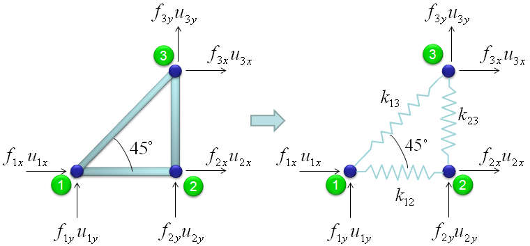
< Example 8 : FEM(Finite Element Method) - Truss Analysis >
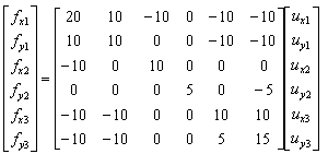
I got the idea of this example from IFEM.Ch01.Slides.pdf, IFEM.Ch02.Slides.pdf, IFEM.Ch03.Slides.pdf (Try google these files and will get further details). The goal in this example is to show the process to construct the stiffness matrix for a simple truss as shown at the left side of the following illustration. You can replace each bar with a spring as shown in the right side of the following illustration. Now you have very similar model to the previous example. But there is very one important difference between this example and previous example. In previous example, we assumed that each node can move only in ONE direction. x direction (horizontal direction), but in this example we give each of the nodes one more freedom. Now each node can move in any way in two dimensional plane. It means the direction of the force applied to each node can be from anywhere in the plane, but as you know wherever the direction is we can describe the force with the two component of forces (horizantal force and vertical foruce) as marked below. "f" represents the force acting on each node and "u" represents the displacement of each nodes as result of the forces acting on the node.
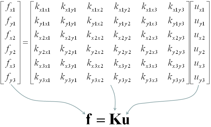
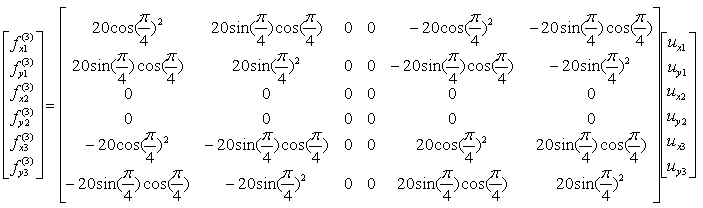
The force and stiffness matrix, displacement relationship is represented as follows and the goal in this example is to go through the steps to fill out the stiffness matrix (K matrix). You may feel a little strange because you have 6 x 6 matrix when you have only three nodes. According to the logic in previous example, you might expect that you would have 3 x 3 matrix since you have only three nodes. The reason why you have much larger matrix than the number of the nodes is that you have to describe the two directional forces for each node.
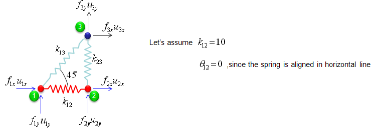
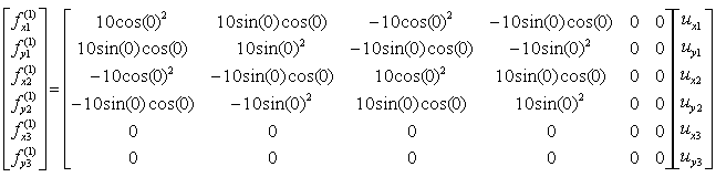
Overall procedure of realizing the matrix (stiffness matrix) is almost same as you saw in previous example. The first step is to split the whole system into each components. The first component is about the two nodes (node 1 and 2). As shown below, these two nodes are connected by single spring marked in red.
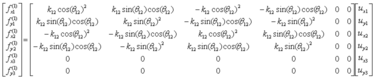
The stiffness values about this spring connecting these two nodes are described as below. (You can refer to the slides that I mentioned at the beginning to understand where these mathematical expression came from. Or just use these expressions).
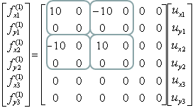
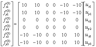
If we assume k12 to be 10 and the angle of the spring from the horizontal line is 0, you can have the following expression.
If you calculate the expressions shown above, you will have the following values.
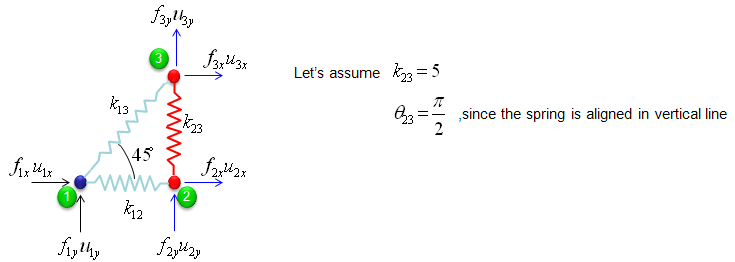
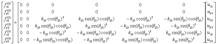
The second component is about the two nodes (node 2 and 3). As shown below, these two nodes are connected by single spring marked in red.
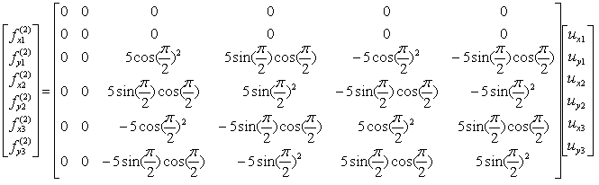
The stiffness values about this spring connecting these two nodes are described as below. (You can refer to the slides that I mentioned at the beginning to understand where these mathematical expression came from. Or just use these expressions).
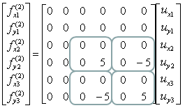
If we assume k23 to be 5 and the angle of the spring from the horizontal line is 90 degree (pi/2), you can have the following expression.
If you calculate the expressions shown above, you will have the following values.
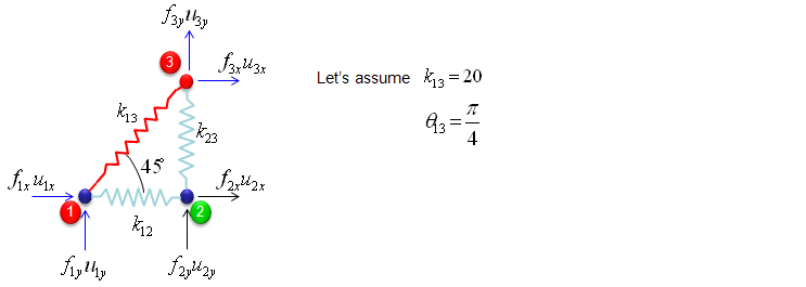
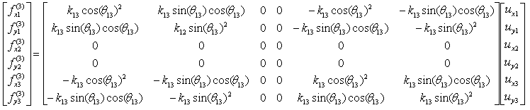
The third component is about the two nodes (node 3 and 1). As shown below, these two nodes are connected by single spring marked in red.
The stiffness values about this spring connecting these two nodes are described as below. (You can refer to the slides that I mentioned at the beginning to understand where these mathematical expression came from. Or just use these expressions).
If we assume k13 to be 20 and the angle of the spring from the horizontal line is 45 degree (pi/4), you can have the following expression.
If you calculate the expressions shown above, you will have the following values.
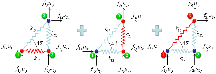
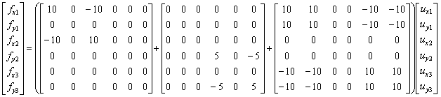
Through the three steps we have done above, you have three stiffness matrix describing each two nodes connected by each spring. The final step is to combine all of these matrix and get a single/combined stiffness matrix.
With summation of the three matrices that we got from previous steps,
you would get the following single matrix.
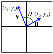
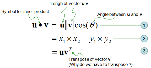
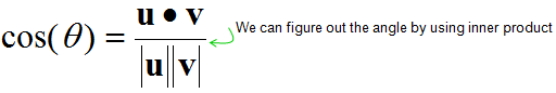
I see two major application of the inner product. One is to figure out the angle between the two vectors as illustrated above. (First, you calculate the inner product using Equation (2) and with the result and equation (1), you can figure out the angle). This angle in turn has additional implication. If this angle is 90 degree(0.5 pi), it means
If this angle is 0 degree, it means
If this angle is between 0 and 90, the value is between min(0) and max value and they are partially dependent to each other.
Second application is nothing to do with geometric meaning, but it is very handy form of mathematical representation of "Sum of Multiplication/Sume of Times" as shown in "Sum of Times" page.
One important thing you have to remember is that the result of inner product of two vectors is a scalar.
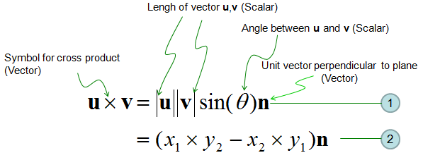
It is pretty complicated process to calculate the cross product in terms of calculation process, but it is not that complicated to understand the geomatrical meaning for it. (Fortunately you don't have to calculate this by your hand. A lot of sotware package out there would do this for you. So what you have to do is just to understand the concept).
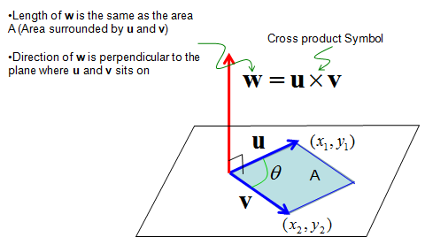
First thing you remember about the cross product is that the result of cross product of two vectors is also a vector (you would remember the result of inner product of two vectors is a scalar). By the definition of vector, it has both direction and size(magnitude).
Then, what is the direction of the resulting vector of cross product ? It is normal (perpendicular) to the plane on which the two vectors sits on. It implies that if you get the cross product of two vector, you will get a vector which is normal to the two input vectors. This is one of the reason why 'cross product' is such a useful tool.
Then, what is the size(magnitude) of the resulting vector of cross product ? It is the area of the area surrounde by the two vectors.
Following is the illustration showing what I described above.
Following is the concept of Cross Product represented in mathematical formula. The calculation shown in equation (2) may look pretty simple, but if the vector goes into higher dimesion the calculation goes exponentially complicated. But as I said, don't worry about this. Software would do it for you.
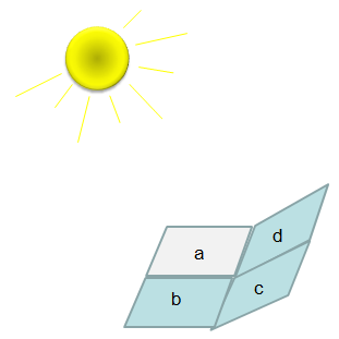
We have learned very two important operations for vectors, inner product and outer product. Combining these two operation we can produce extremely useful tool. This tool is so widely used that it has it's own name, called 'Scalar Triple Product'.
Let me give you a situation where we can use the concept of Scalar Triple Product. We have a multiple planes connected to each other with different tilt and light (sun) is shining over them as shown below.
Now let's think about which plane (plate) would have the strongest light. Any idea ? Intuitively you would guess that the plate getting the light closer to right angle (perpendicular to the plane/plate).
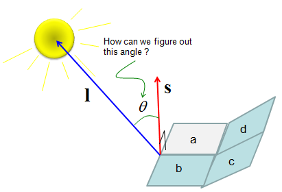
How can we know how closer to the right angle a plate is getting the light ? The idea is like this. i) Draw a vector which is perpendicular to the plane/plate(Let's label this vector as s). ii) Draw a vector which connector a corner of the plate to the center of the light(Let's lavel this vector as l ) iii) Calculate the angle between the two vectors (s and l). If this angle closer to 0, it means the it is getting the light closer to the right angle.
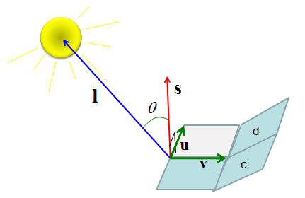
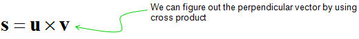
Now let translate this procedure into mathematical forms. First, we have to get a vector which is perpendicular (normal) to a plane (plate). Any idea on this ? This is where you can use the concept of 'Cross Product'. If you draw two vectors starting a corner of the plate running along the sides as marked in green arrow shown below. The cross product of the two vectors would give you a vector which is perpendicular to the plate. Now the next step would be to figure out the angle between the angle between vector s and l. This is what Inner Product is used for.
Following is the mathematical description for the procedures explained above.
First, get the vector s which is perpendicular to a plate by 'Cross Product' as shown below.
Second, by a little bit of rearrangement of Inner Product equation, you can get the angles between the vector s and vector l.
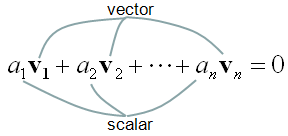
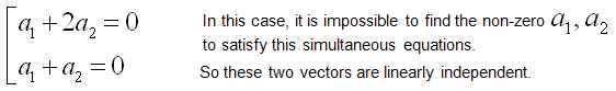
Linear Independence is an indicator of showing the relationship among two or more vectors. Putting it simple, "Linear Independence" imply "No correlation between/among the vectors". The mathematical definition of linear independence is as follows.
Like many other mathematical definitions, it is hard to grasp a clear understanding without going through examples. Let's suppose we have two vectors and want to check if the two vectors are 'linearly independent" or not. Applying the two vectors into the definition of linear independecy, we can express it as follows.
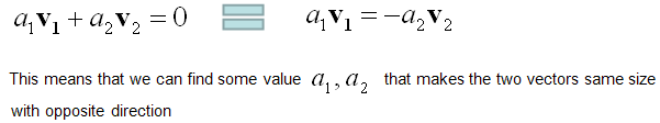
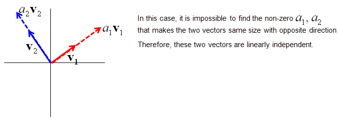
If I assume the two vectors are 2x1 vector, we can describe each component of the above mathemtical expressions as follows. As you see in this example, if we have only two vectors and the direction of vectors are different, they are 'linearly independent'.
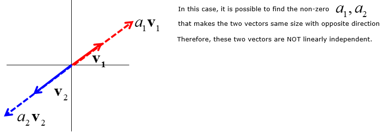
If the two vectors are aligned in the same direction or in completely opposite direction (180 degree difference), we can easily find a non-zero a1,a2 value to make these two vectors 'NOT linear independent'.
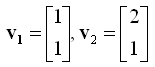
Now let's see another example showing concrete numbers. Let's assume that we have two vectors as shown below.
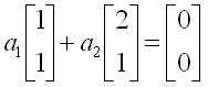
Let's plug these two vector into the definition of linear independence. It becomes as follows.
If we plug the values into the expression, we get following expression.
Now the question is "Can we find any non-zero a1, a2 to satisfy this equation ?" and the result and the conclusion comes as follows.
Then the last question would be "Why the linear independency is important ?", "How do we utilise this concept ?". The importance of this concept would be for calculating the Rank of a matrix or for investigating the existence of solution of a simultaneous equation.
Intuitive Property of a Matrix
My own image for a matrix is a kind of machine that is doing things as follows. As you see in the illustration, Matrix is taking in a shape (geometrical shape/object) and transform (change shape) them in mainly three different way as follows. i) Scale (magnify or shrink) ii) Rotate iii) Skew In reality, a matrix can do more than one type of transformation like "Scale and Skew", "Scale and Rotate and Skew" etc. I will talk about this kind of transformation in this section and I hope you can have some intuitive understanding of the propery of a matrix since it can be visualized as in this section.
I think one of the best way to understand the characteristics of a Matrix is to apply it for an shape in a graphical coordinates and observe the result. Of course, there would be a certain limitation in this method since we can only visualize three dimensional shape and as a result the dimension of the matrix we can visualize would be 3 x 3 (or 4 x 4 in some cases). But if you build up a solid intuitive understanding of a properties of a matrix in this way, you can easily extend the understanding to any size of the matrix and, more importantly, you can understand more easily a mathematical model represented in the matrix format.
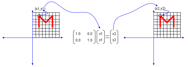
I will use a shape in two dimensional coordinate and 2 x 2 matrix applying to the shape on the coordinate. Here you see coordinates labeled (x1,y1) and (x2,y2). (x1,y1) represents each points before it is transformed by the matrix and (x2,y2) is the new points after (x1,y1) is transformed by the matrix.
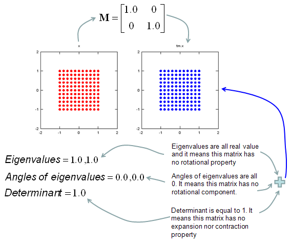
Let's look at the first case. The first matrix is what we call Identity Matrix which has the value '1' in all the elements on diagonal line running from left top to right bottom and all the other elements are set to be '0'. What is the result of the transformation of a shape transformed by the Identity Matrix ? The answer is "No change".
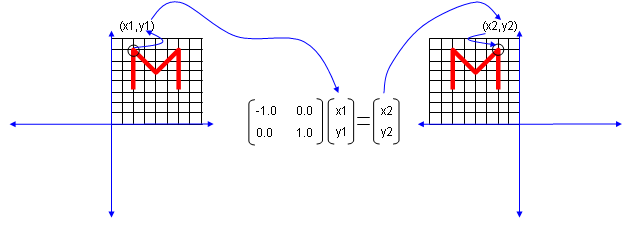
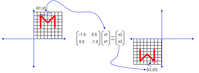
Next look at another matrix shown below. This matrix also looks similar to diagonal matrix but not exactly same. The difference is that the first element on the diagonal line is '-1' in stead of '1'. What is the result ? The shape is flipped around y axis.
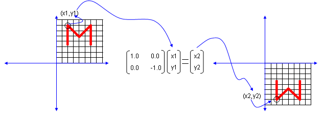
Next look at another matrix shown below. This matrix also looks similar to diagonal matrix but not exactly same. The difference is that the second element on the diagonal line is '-1' in stead of '1'. What is the result ? The shape is flipped around x axis.
Next look at another matrix shown below. In this case, all the elements on the diagonal lines is set to be '-1' instead of '0'. What is the result ? It became reflected around the point (0,0). You can interpret this in two steps. At the first step, the shape is flipped around y axis. and at the second step the shape is fliped around x axis.
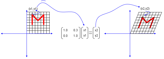
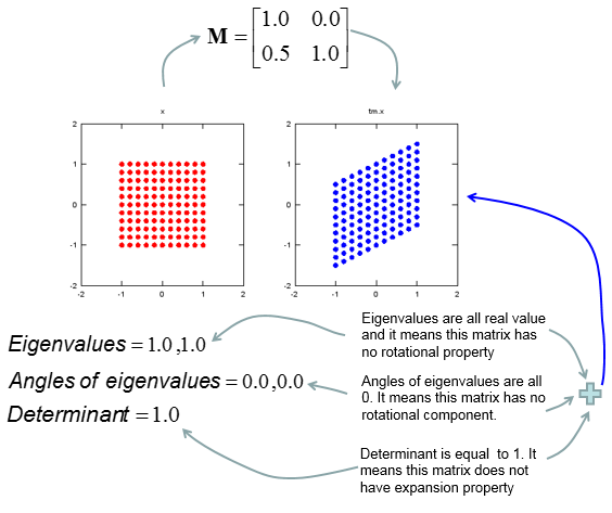
Now let's look at another matrix as shown below. This time you see all '0's on the diagonal line and now you see a non-zero value out side of diagonal line. What is the result ? The image shears.
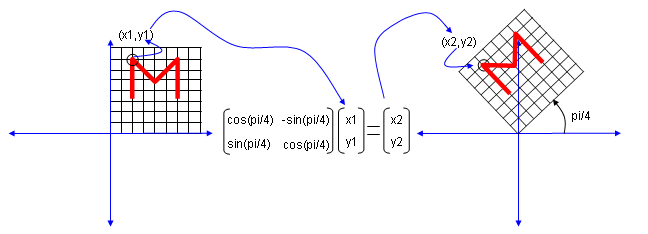
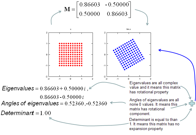
Now let's look at another matrix as shown below. This time you see the non-zero value in all the elements. This is tricky to analyze since these matrix can do almost everything described above.. but if the numbers in the elements can be represented as trigonometrix functions in the following format. This matrix can rotate the image as shown below.
Actually this is only a few of the examples.. you can try any numbers in the matrix and apply to some shape and try to correlate those numbers to the result of the transformation until you build up your own intuition of figuring out the characteristics of a matrix.
One of the most useful/important but very hard to understand the practical meaning would be the concept of Eigenvector and Eigenvalue. You can easily find the mathematical definition of eigenvalue and eigenvector from any linear algebra books and internet surfing.
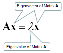
I will start with the samething, i.e mathematical definition. Mathematical definition of Eigenvalue and eigenvectors are as follows.
Let's think about the meaning of each component of this definition. I put some burbles as shown below.
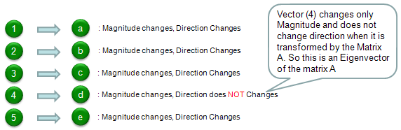
When a vector is transformed by a Matrix, usually the matrix changes both direction and amplitude of the vector, but if the matrix applies to a specific vector, the matrix changes only the amplitude (magnitude) of the vector, not the direction of the vector. This specific vector that changes its amplitude only (not direction) by a matrix is called Eigenvector of the matrix.
Let me try explaining the concept of eigenvector in more intuitive way. Let's assume we have a matrix called 'A'. We have 5 different vectors shown in the left side. These 5 vectors are transformed to another 5 different vectors by the matrix A as shown on the right side. Vector (1) is transformed to vector (a), Vector (2) is transformed to vector (b) and so on.
Compare the original vector and the transformed vector and check which one has changes both its direction and magnitude and which one changes its magnitude ONLY. The result in this example is as follows. According to this result, vector (4) is the eigenvector of Matrix 'A'.
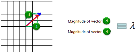
I hope you clearly understand the meaning of eigenvectors. Now we know eigenvector changes only its magnitude when applied by the corresponding matrix. Then the question is "How much in magnitude it changes ?". Did it get larger ? or smaller ? exactly how much ? The indicator showing the magnitude change is called Eigenvalue. For example, if the eigenvalue is 1.2, it means that the magnitude of the vector gets larger than the original magnitude by 20% and if the eigenvalue is 0.8, it means the vector got smaller than the original vector by 20 %. The graphical presentation of eigenvalue is as follows.
Now let's verbalize our Eigenvector and Eigenvalue definition.
Matrix multiplied to its Eigenvector is same as the Eigenvalue multiplied to its Eigenvector.
Then very important question would be "Why we need this kind of Eigenvector / Eigenvalue ?" and "When do we use Eigenvector / Eigenvalue ?".
The answer to this question cannot be done in a short word, the best way is to collect as many examples as possible to use these eigenvector/eigenvalues. You can find one example in this page, the section Geometric/Graphical Meaning of Eigenvalue and Determinant
i) When you have a situation in which you have to multiply a matrix to a vector repeatedly (for example, let's assume that you have to multiply a matrix 100 times), it would require a lot of calculation. But you can predict this result just by looking at the eigenvalues without doing 100 times matrix multiplication. (You can see this kind of cases a lot in stochastics). ii) You can use the eigenvectors and eigenvalues to get the solution of linear differential equations (see here). iii) In computer graphics, a matrix is multiplied to several hundreds of points (vectors) to change the shape of an image represented by the points. By analyzing the eigenvectors of the matrix (transformation matrix), you can predict the overall result of the change of the shape without doing the several hundreds matrix x vector multiplication. (see here)
For more examples, refer to http://wiki.answers.com/Q/What_are_the_applications_of_Eigenvalue_and_eigenvector_in_Engineering
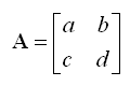
To be honest how to describe the mathemtical definition of a Matrix that can apply to any size of matrix. As you may learned in High school math or linear algegra course, the definition of Determiant for 2 x 2 matrix as follows is very simple as shown below.
Determinant of A = ad-bc
But this kind of definition would not help much about understanding the real meaning of determinants and the calculation process gets exponentially complicated as the size of the matrix gets larger. If the size of matrix is equal to or greater than 4 x 4, it would be almost impossible to calculate it by hand.
So I would focus more on explaining the practical meaning of the determinants rather than calculation process.
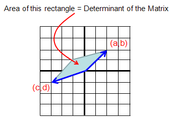
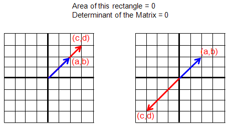
Practical meaning of Determinant of matrix of 2 x 2 is as follows. It is the area of the shape enclosed by the two vectors which are made out of each row of the matrix.
In some cases as follows, the determinants gets 0.
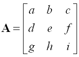
Let's look into the case of 3 x 3 matrix as follows.
The practical meaning of Determinant of matrix is the volume of the object defined by the three vectors which is made out of each row of the matrix.
If the size of matrix gets equal to/higher than 4 x 4, it would be difficult to visualize the definition geometrically as above, but I hope you can have your own image at least.
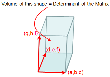
Real importance of Determinant can be described as follows. You can understand basic characteristics of a matrix from determinant. When you apply a Matrix to vectors, you can make pretty reasonable guess just by looking at Determinant without doing all the calculation. If the process requires only one time calculation (e.g, one time multiplication of Matrix and vector) it would be no problem to perform the calculation, but if you have to do many times it would be handy to make a inference of the result from Determinant rather than doing all the 'matrix x vector' multiplication.
You will see some examples of using the determinants of Matrix in Geometric/Graphical Meaning of Eigenvalue and Determinant
Rank is an indicator that shows how many of the vectors comprising a matrix are linearly independent to each other. For example, let's suppose we have a matrix as follows.
Let's take each row of the matrix and construct vectors as follows. (These vectors are called 'row vector')
Now the question is how many of these vectors are linearly independent to each other ? The answer to this question is the Rank of the matrix.
(Refer to "Linear Independent" definition)
Geometric/Graphical Meaning of Eigenvalue and Determinant
My own image for a matrix is a kind of machine that is doing things as follows. As you see in the illustration, Matrix is taking in a shape (geometrical shape/object) and transform (change shape) them in mainly three different way as follows. i) Scale (magnify or shrink) ii) Rotate iii) Skew In reality, a matrix can do more than one type of transformation like "Scale and Skew", "Scale and Rotate and Skew" etc.
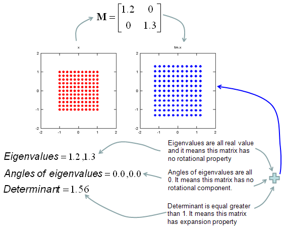
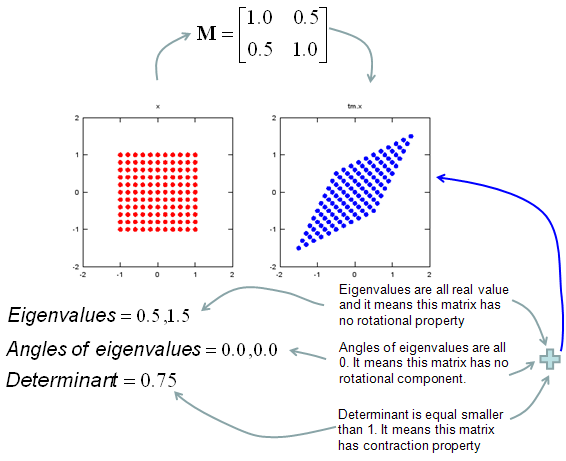
In this sections, I will show you how a matrix transforms a given image (a set of dots). For each example, I transformed 100 dots.. it means that I had to calulate "A x v" type of vector multiplication 100 times. It would have been almost undoable if I had to do it with pen and paper unless I had an extraordinary patience. (Definately I am not such a patient person -:)). Fortunately, I have a software with which I can do this kind of things relatively easy. Following is the source script that I created for these examples. You can apply whatever 2 x 2 matrix just by changing "tm = [1.0 0.0;0.5 1.0]" part. There are other very important points in these examples. For each example, I (matlab source script) calculated the following values and I put down a short comments on what kind of information you can get from these values. i) Eigenvalue ii) Angle of each Eigenvalue iii) Determinant
When you were learning Eigenvalue, Determinant.. the first question you might have would be "What are these for ?" "Why do we have to calculate these values ?". This is one of the examples in which you can use eigenvalues and determinant in very useful way. If there is no computer and I am asked to get overall image of the transformation of 100 points as in this example, I would definitely calculate eigenvalue and determinant and make a reasonable guess of the final result, rather than trying to 100 times of "A x v" calculation. This kind of interpretation of Eigenvalue and Determinant is not only for geometrical transformation, but also can be useful almost any system represented as a Matrix system (e.g, Control System, Stochastics, Structure Analysis etc). So I strongly recommend you to go through in very detail and try a lot of example matrix with the Matlab/Octave script and get some intuitive understandings of your own.
ptList_x=[]; ptList_y=[];
for y=-1.0:0.2:1.0 for x=-1.0:0.2:1.0 ptList_x=[ptList_x x]; ptList_y=[ptList_y y]; end end
ptList_v = [ptList_x' ptList_y']; ptList_v = ptList_v';
tm = [1.0 0.0;0.5 1.0] tm_eigenvalue = eig(tm) Angle_of_eigenvalues = arg(tm_eigenvalue) tm_determinant = det(tm)
ptList_v_tm = tm * ptList_v; ptList_v_tm_x = ptList_v_tm(1,:); ptList_v_tm_x = ptList_v_tm_x'; ptList_v_tm_y = ptList_v_tm(2,:); ptList_v_tm_y = ptList_v_tm_y';
subplot(1,2,1); plot(ptList_x,ptList_y,'ro','MarkerFaceColor',[1 0 0]);axis([-2 2 -2 2]);title('x');daspect([1 1]); subplot(1,2,2); plot(ptList_v_tm_x,ptList_v_tm_y,'bo','MarkerFaceColor',[0 0 1]);axis([-2 2 -2 2]);title('tm.x');daspect([1 1]);
In the above section, you saw some examples of how a matrix can transform a shape in a coordinate. But all the elements in the matrix and the numbers representing a point in a coordinate were real numbers. In this section, you would see examples where complex numbers are used in both matrix and coordinate. As you may see in complex number section, the operation of the complex number itself has some geometric transformation properties. Therefore, the final outcome of the transformation of complex coordinate and complex matrix are even more complicated. Only real practice on your own would give you the real meaning of those transformation.
This kind of transformation are used pretty often in MIMO (Multiple Input Multiple Output) in wireless communication.
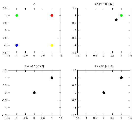
Let's directly jump into some examples. Following is a Matlab/Octave code that I wrote. v1, v2, v3, v4 are a complex number representing a constellation point in I/Q coordinate. m1,m2,m3 is a complex transformation matrix. c1, c2 can be any two complex numbers selected from {v1, v2, v3, v4}. Just try this code and observe the result. Change any of v1,v2,v3,v4, c1,c2, m1,m2,m3 and rerun the code. Repeat this process until your brain get the overall pictures of how this transformation work.
v1 = 1 + j; v2 = -1 + j; v3 = -1 - j; v4 = 1 - j;
c1 = v1; c2 = v2;
m1 = 1/sqrt(2).*[1 0; 0 1] m2 = 1/2.*[1 1; 1 -1] m3 = 1/2.*[1 1; j -j]
m1_c12 = m1 * [c1;c2] m2_c12 = m2 * [c1;c2] m3_c12 = m3 * [c1;c2]
subplot(2,2,1); plot(real(v1), imag(v1),'ro','MarkerFaceColor',[1 0 0], 'MarkerSize',10, ... real(v2), imag(v2),'go','MarkerFaceColor',[0 1 0], 'MarkerSize',10, ... real(v3), imag(v3),'bo','MarkerFaceColor',[0 0 1], 'MarkerSize',10, ... real(v4), imag(v4),'yo','MarkerFaceColor',[1 1 0], 'MarkerSize',10); axis([-1.5 1.5 -1.5 1.5]); title('A');
subplot(2,2,2); plot(real(c1), imag(c1),'ro','MarkerFaceColor',[1 0 0], 'MarkerSize',10, ... real(c2), imag(c2),'go','MarkerFaceColor',[0 1 0], 'MarkerSize',10, ... real(m1_c12), imag(m1_c12),'ko','MarkerFaceColor',[0 0 0], 'MarkerSize',10); axis([-1.5 1.5 -1.5 1.5]); title('B = m1 * [c1;c2]');
subplot(2,2,3); plot(real(c1), imag(c1),'ro','MarkerFaceColor',[1 0 0], 'MarkerSize',10, ... real(c2), imag(c2),'go','MarkerFaceColor',[0 1 0], 'MarkerSize',10, ... real(m2_c12), imag(m2_c12),'ko','MarkerFaceColor',[0 0 0], 'MarkerSize',10); axis([-1.5 1.5 -1.5 1.5]); title('C = m2 * [c1;c2]');
subplot(2,2,4); plot(real(c1), imag(c1),'ro','MarkerFaceColor',[1 0 0], 'MarkerSize',10, ... real(c2), imag(c2),'go','MarkerFaceColor',[0 1 0], 'MarkerSize',10, ... real(m3_c12), imag(m3_c12),'ko','MarkerFaceColor',[0 0 0], 'MarkerSize',10); axis([-1.5 1.5 -1.5 1.5]); title('D = m3 * [c1;c2]');
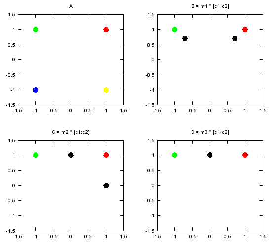
As the first example, I selected v1 and v2 as the two numbers to be transformed by the matrix. Following is the numerical result of the transformation. m1_c12 is the result of transformation of (c1,c2) by the matrix m1. m2_c12 is the result of transformation of (c1,c2) by the matrix m2. m3_c12 is the result of transformation of (c1,c2) by the matrix m3.
c1 = v1; c2 = v2; m1_c12 =
0.70711 + 0.70711i -0.70711 + 0.70711i
m2_c12 =
0 + 1i 1 + 0i
m3_c12 =
0 + 1i 0 + 1i
Following is the graphical representation of the result of this transformation. Graph A shows the four complex numbers v1,v2,v3,v4 in I/Q coordinate. Red = v1 Green = v2 Blue = v3 Yellow = v4 Black = the result of transformation of (c1,c2) by m1, m2, m3
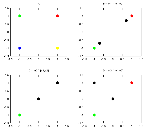
In the second example, I selected v1 and v3 as the two numbers to be transformed by the matrix. Following is the numerical result of the transformation. m1_c12 is the result of transformation of (c1,c2) by the matrix m1. m2_c12 is the result of transformation of (c1,c2) by the matrix m2. m3_c12 is the result of transformation of (c1,c2) by the matrix m3.
c1 = v1; c2 = v3;
m1_c12 =
0.70711 + 0.70711i -0.70711 - 0.70711i
m2_c12 =
0 + 0i 1 + 1i
m3_c12 =
0 + 0i -1 + 1i
Following is the graphical representation of the result of this transformation. Graph A shows the four complex numbers v1,v2,v3,v4 in I/Q coordinate. Red = v1 Green = v2 Blue = v3 Yellow = v4 Black = the result of transformation of (c1,c2) by m1, m2, m3
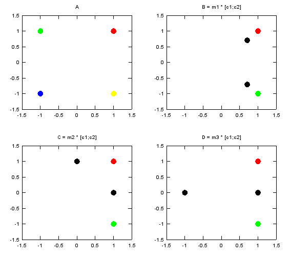
In the third example, I selected v1 and v4 as the two numbers to be transformed by the matrix. Following is the numerical result of the transformation. m1_c12 is the result of transformation of (c1,c2) by the matrix m1. m2_c12 is the result of transformation of (c1,c2) by the matrix m2. m3_c12 is the result of transformation of (c1,c2) by the matrix m3.
c1 = v1; c2 = v4;
m1_c12 =
0.70711 + 0.70711i 0.70711 - 0.70711i
m2_c12 =
1 + 0i 0 + 1i
m3_c12 =
1 -1
Following is the graphical representation of the result of this transformation. Graph A shows the four complex numbers v1,v2,v3,v4 in I/Q coordinate. Red = v1 Green = v2 Blue = v3 Yellow = v4 Black = the result of transformation of (c1,c2) by m1, m2, m3
In the fourth example, I selected v1 and v1 again as the two numbers to be transformed by the matrix. Following is the numerical result of the transformation. m1_c12 is the result of transformation of (c1,c2) by the matrix m1. m2_c12 is the result of transformation of (c1,c2) by the matrix m2. m3_c12 is the result of transformation of (c1,c2) by the matrix m3.
c1 = v1; c2 = v1;
m1_c12 =
0.70711 + 0.70711i 0.70711 + 0.70711i
m2_c12 =
1 + 1i 0 + 0i
m3_c12 =
1 + 1i 0 + 0i
Following is the graphical representation of the result of this transformation. Graph A shows the four complex numbers v1,v2,v3,v4 in I/Q coordinate. Red = v1 Green = v2 Blue = v3 Yellow = v4 Black = the result of transformation of (c1,c2) by m1, m2, m3
Decomposition is a method of splitting a matrix into multiplication of multiple matrix in the following form.
M = AB..N
How many matrix you split M into and the characteristics of splitted matrix varies depending on each specific decomposition method. Actually 'breaking one thing into multiple other things' is one of the most common techniques in mathematics. For example, we often break a number into multiples of other numbers as follows.
15 = 2 x 3 x 5
We also break a polynomial into the multiples of other polynomials as shown below.
x^4 - 5 x^3 - 7 x^2 + 29 x + 30 = (x+2)(x+1)(x-3)(x-5)
Question is "Why we do this kind of break down ?". Sometimes we may do this kind of thing just for mathematical fun or curiosity, but in most case (especially in engineering area) we do this because we can get some benefit from it. For example, if you are asked to plot a graph for x^4 - 5 x^3 - 7 x^2 + 29 x + 30, you may have to do a lot of work (a lot of punching keys on your pocket calculator), but if you break the polynomial into (x+2)(x+1)(x-3)(x-5), you would be able to overal shape of the graph without doing even single calculation. Samething applies to Matrix decomposition. We decompose a Matrix into multiple other matrices because there are advantages doing it. What kind of benefit you can get from the matrix decomposition ? We can think of mainly two advantages
Then you may ask "Why I don't see this kind of benefit in the linear algebra course ?". "It just look like trying to make simple things more complex.", "It is seems to be designed just to give headache to students". Mainly two reasons for this
However if you are given a matrix equation with a huge matrix (like 1000000 x 1000000), then you would start seeing the benefit of doing decomposition. Of course, you cannot decompose 1000000 x 1000000 by hand. You have to use computer. Then you may ask "If I use computer, why bother to decompose ? Computer would do the calculation directly from the original matrix". But in reality it is not. If the size of matrix is very large, there would be huge differences between with and without decomposition even for the high performance computer.
See http://en.wikipedia.org/wiki/Matrix_decomposition and see LU Decomposition in this page as a specific example. (I will keep adding more examples when I have chance)
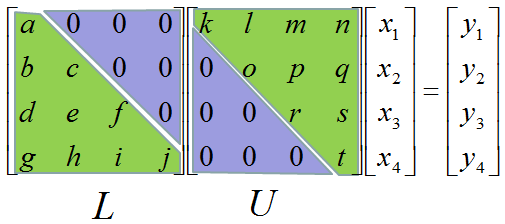
LU decomposition is a method to split (decompose) a matrix into two matrix product. One of these two matrix(the first part) is called 'L' matrix meaning 'Lower diagonal matrix' and the other matrix(the second part) is called 'U' matrix meaning 'Upper diagonal matrix'. Simply put, LU decomposition is a process to convert a Matrix A into the product of L and U as shown below.
A = LU
I would not explain about how you can decompose a matrix into LU form. The answer is "Use software" -:). I would talk about WHY.
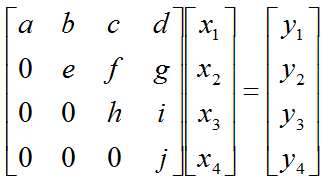
Let's assume that we have a matrix equation (Linear Equation) as shown below.
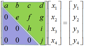
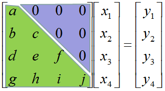
Don't look into each elements yet. Just get around 100 steps back away from this and look at the overall pattern of the matrix. Can you see a pattern as shown below ? You see two area marked as triangles. Green triangle shows all the elements from diagonal line and upper diagonal part. The elements in this triangle is non-zero values. Violet triangle shows the elements of lower diagonal part which is all zero.
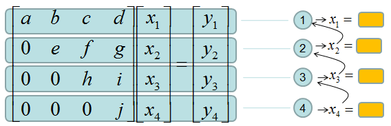
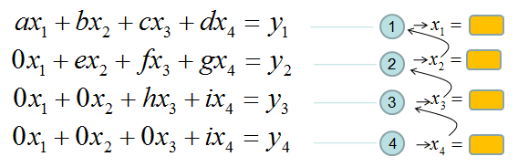
This form of matrix is called 'U' form matrix, meaning 'Upper diagonal matrix'. Why this is so special ? It is special because it is so easy to solve the equation. Now let's think about how we can solve this equation. Let's look the last row (4th row in this case). How can I figure out the value for x4 ? You would get it right away because there is only x4 term and j and y4 are known values. Once you get x4 and plug in the x4 value into row 3, then you would get x3 value. Once you get x3 and plug in the x3 value into row 2, then you would get x2 value. Once you get x2 and plug in the x2 value into row 1, then you would get x1 value.
If it is not clear with you, it would be a little clearer if you convert the matrix equation into simultaneous equation as shown below. Start from the last equation and get x4 first and repeat the process described above.
If this process is still unclear,just play with real numbers. Put any numbers for a,b,c,d,e,f,g,h,i,y1,y2,y3,y4 and try to get x1,x2,x3,x4 as explained above.
If you tried this as explained, one thing you would notice would be "It is so simple to find the solution x1,x2,x3,x4". Just compare this process with what you experienced with general matrix equation solving process you did in your high school math or linear algebra class.
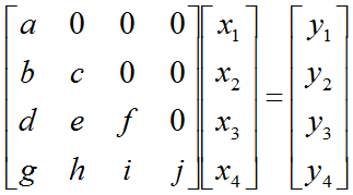
Now let's look into another example of matrix equation as shown below.
Now you would know what I will say. In this case, all the elements along the diagonal line and Lower part of diagonal line is non-zero values. All the values above the diagonal line is all zero. This form is called 'L' form meaning 'Lower diagonal matrix'.
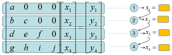
Why this is so special ? It is special because it is so easy to solve the equation. Now let's think about how we can solve this equation. Let's look the first row (the first row in this case). How can I figure out the value for x1 ? You would get it right away because there is only x1 term and a and y1 are known values. Once you get x1 and plug in the x1 value into row 2, then you would get x2 value. Once you get x2 and plug in the x3 value into row 3, then you would get x3 value. Once you get x3 and plug in the x2 value into row 4, then you would get x4 value.
If it is not clear with you, it would be a little clearer if you convert the matrix equation into simultaneous equation as shown below. Start from the first equation and get x1 first and repeat the process described above.
If this process is still unclear,just play with real numbers. Put any numbers for a,b,c,d,e,f,g,h,i,y1,y2,y3,y4 and try to get x1,x2,x3,x4 as explained above.
If you tried this as explained, one thing you would notice would be "It is so simple to find the solution x1,x2,x3,x4". Just compare this process with what you experienced with general matrix equation solving process you did in your high school math or linear algebra class.
Now let's suppose we have a matrix as shown below. Here all the elements in the matrix is non-zero values.
Now let's assume we can convert this matrix equation into following form. (Don't worry about HOW, just assume you can do this somehow). You already know that this form would make it easier to solve the equation.
Try this example that I found from web. (If the link is missing, try here).
Now you may say.. "You always say 'don't worry about how to solve. just use computer software'". If I use the computer software, why do I have to worry about this kind of conversion. Computer software would not have any problem to solve the equation even with the original form without LU decomposition. You are right, the computer program would not have any problem with original form.But the amount of time for the calculation is much shorter with LU decomposed form than the original form. When the size of matrix, this time difference would be negligiable, but if the size is very huge (e.g, 10000 x 10000) the time difference would be very huge. If you've done a computer science, you would be familiar with Big O notation to evaluate the computation time. Try compare the computation time for the original matrix form and LU decomposed form. If you are not familiar with this notation, just trust me -:). Following two YouTube tutorial would give you some insight of LU decomposition including computation time.
I tried to visualize most of the concept in this engineering math pages so that it would give you some intuitive understanding and provide a visual cheat sheet. Even though you think you already understood something, that understanding and memories fades away very quickly but if you gives yourself just brief movent of visual Que of those concept while is fading away, it would refresh your memory and solidify your understanding. But there are some of the concepts which came out of purely mathemtical logics and very hard to visualize it. Also very hard to explain intuitively. Many of the concepts I will explain from now would fall into this group. So it would easily get your bored if you just try to read through. So my recommendation is "Don't try to read this or understand everything in detail now. Try to pick any engineering application in which they often use this concept/notation. Use this part as a quick reference to understand the mathematical model of the application that you picked".
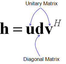
For example, my personal motivation for this section was as follow. When I first read literature about MIMO (Mutiple Input Multiple Output) in mobile communication system, I came across a famous equation as follows. (I would not explain about the meaning of this equation now. Just take a look at the equation itself).
You see the term called "unitary matrix", "singular matrix" and strange looking notation v^H here. You may dimmly recall that you have learned these terms in your linear algebra course but have no idea of the details now. So I start gooling and reading Wikipedia about these terms and I came across another bunch of terms like orthogonal matrix, congjugate transpose, Hermitian Congugate etc. Struggling through tons of pages back and forth, finally I thought I would need to understand all of these building block concepts first to read the literature that I am interested in.
Conjugate Transpose, Hermitian Conjugate
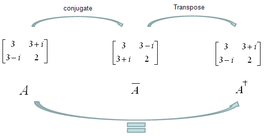
Conjugate Transpose is literaly as it says. Get the complex conjugate of the matrix and transpose it. As illustrated below. Especialy try to get familiar with mathemtical symbols for this (final result). This is also called Hermitian conjugate.
Hermitian Matrix is a special matrix, which is same as its conjugate transpose as expressed below.
One example is as follows.
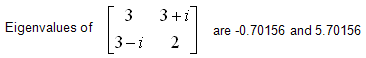
One of the important characteristics of Hermitian Matrix is that Eigenvalues of all Hermitian Matrix are all real as shown in the following example.
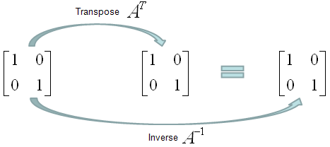
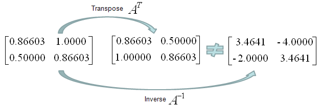
Orthogonal Matrix is a special form of matrix that meets the following criteria saying "Transpose of the matrix is same as the inverse of the matrix".
A couple of examples would give you better understanding. Is following matrix (the matrix in the left). Yes it is because its transpose and inverse are same.
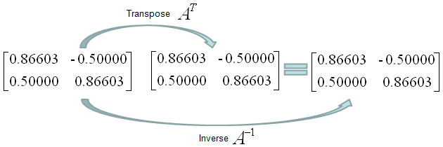
Is following matrix (the matrix in the left) orthogonal. Yes it is because its transpose and inverse are same.
Is following matrix (the matrix in the left) orthogonal. No it is not because its transpose and inverse are not same.
Orthonormality is a characteristics of the relations among two of more vectors. It is defined by following characteristics.
Singular Matrix is defined as a Matrix which does not have matrix inverse. It means
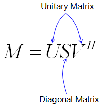
Unitary Matrix is a special kind of complex square matrix which has following properties. (U in the following description represents a unitary matrix)
Singular Value Decomposition(SVD)
Singluar Value Decomposition is a technique which decompose a matrix into three components as follows.
As you recall from the early part of this page, a matrix can magnify or rotate or shear the set of dots(points in a coordinate). If M is square matrix, SVD become a method to convert the whole transformational process into rotational component, magnifying component and shear component. U and V* (V Hermitian) performs 'rotational' operation and S performs 'Scaling' operation.
Followings are some characteristics of these decomposed matrices.
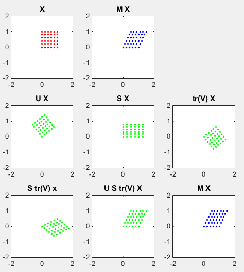
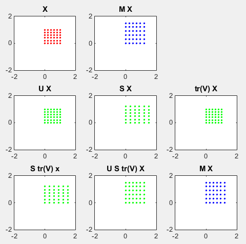
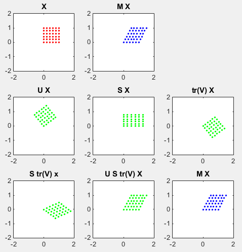
A graphical presentation of SVD is as follows. (I also posted the Octave/Matlab script that I wrote for this illustration and playwith various other matrix('tm' in the script) and see the result until get some intuitive feeling about this process).
Look at the graphs on the top row. The red dots on left graph are transformed by the matrix M to be the blue dots on right graph. Look at the graph on the middle row. The dots on left graph is the result of transforming M with the matrix U. You can see here that the area of the original rectangle(array of red dots) does not changes, but it get rotated. The dots on the graph in the middle is the result of transforming M with the matrix S. You don't see any rotation here, but you see the original rectangle (array of red dots) get extended in x direction and contracted in y direction. The dots on right graph is the result of transforming M with the matrix V*(V Hermitian). You can see here that the area of the original rectangle(array of red dots) does not changes, but it get rotated.
ptList_x=[]; ptList_y=[];
for y=-1.0:0.2:1.0 for x=-1.0:0.2:1.0 ptList_x=[ptList_x x]; ptList_y=[ptList_y y]; end end
ptList_v = [ptList_x' ptList_y']; ptList_v = ptList_v';
tm = [1.25 1;0.2 0.9] [U,S,V]=svd(tm)
ptList_v_tm = tm * ptList_v; ptList_v_tm_x = ptList_v_tm(1,:); ptList_v_tm_x = ptList_v_tm_x'; ptList_v_tm_y = ptList_v_tm(2,:); ptList_v_tm_y = ptList_v_tm_y';
ptList_v_tm_u = U * ptList_v; ptList_v_tm_u_x = ptList_v_tm_u(1,:); ptList_v_tm_u_x = ptList_v_tm_u_x'; ptList_v_tm_u_y = ptList_v_tm_u(2,:); ptList_v_tm_u_y = ptList_v_tm_u_y';
ptList_v_tm_s = S * ptList_v; ptList_v_tm_s_x = ptList_v_tm_s(1,:); ptList_v_tm_s_x = ptList_v_tm_s_x'; ptList_v_tm_s_y = ptList_v_tm_s(2,:); ptList_v_tm_s_y = ptList_v_tm_s_y';
ptList_v_tm_v = (conj(V)') * ptList_v; ptList_v_tm_v_x = ptList_v_tm_v(1,:); ptList_v_tm_v_x = ptList_v_tm_v_x'; ptList_v_tm_v_y = ptList_v_tm_v(2,:); ptList_v_tm_v_y = ptList_v_tm_v_y';
ptList_v_tm_vs = (conj(V)') * S * ptList_v; ptList_v_tm_vs_x = ptList_v_tm_vs(1,:); ptList_v_tm_vs_x = ptList_v_tm_vs_x'; ptList_v_tm_vs_y = ptList_v_tm_vs(2,:); ptList_v_tm_vs_y = ptList_v_tm_vs_y';
ptList_v_tm_usv = U * S * (conj(V)') * ptList_v; ptList_v_tm_usv_x = ptList_v_tm_usv(1,:); ptList_v_tm_usv_x = ptList_v_tm_usv_x'; ptList_v_tm_usv_y = ptList_v_tm_usv(2,:); ptList_v_tm_usv_y = ptList_v_tm_usv_y';
subplot(3,3,1); plot(ptList_x,ptList_y,'ro','MarkerFaceColor',[1 0 0]);axis([-2 2 -2 2]);title('x'); subplot(3,3,2); plot(ptList_v_tm_x,ptList_v_tm_y,'bo','MarkerFaceColor',[0 0 1]);axis([-2 2 -2 2]);title('USV.x');
subplot(3,3,4); plot(ptList_v_tm_u_x,ptList_v_tm_u_y,'go','MarkerFaceColor',[0 1 0]);axis([-2 2 -2 2]);title('U.x'); subplot(3,3,5); plot(ptList_v_tm_s_x,ptList_v_tm_s_y,'go','MarkerFaceColor',[0 1 0]);axis([-2 2 -2 2]);title('S.x'); subplot(3,3,6); plot(ptList_v_tm_v_x,ptList_v_tm_v_y,'go','MarkerFaceColor',[0 1 0]);axis([-2 2 -2 2]);title('V.x');
subplot(3,3,9); plot(ptList_v_tm_v_x,ptList_v_tm_v_y,'go','MarkerFaceColor',[0 1 0]);axis([-2 2 -2 2]);title('V.x'); subplot(3,3,8); plot(ptList_v_tm_vs_x,ptList_v_tm_vs_y,'go','MarkerFaceColor',[0 1 0]);axis([-2 2 -2 2]);title('SV.x'); subplot(3,3,7); plot(ptList_v_tm_usv_x,ptList_v_tm_usv_y,'go','MarkerFaceColor',[0 1 0]);axis([-2 2 -2 2]);title('USV.x');
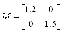
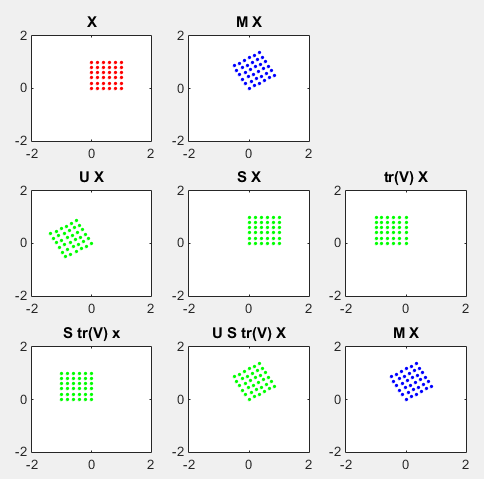
Let's look into another example shown below.
Look at the graphs on the top row. The red dots on left graph are transformed by the matrix M to be the blue dots on right graph. Look at the graph on the middle row. The dots on left graph is the result of transforming M with the matrix U. You can see here that the area of the original rectangle(array of red dots) does not changes, and it does not get rotated either(it means that the matrix M does not have any rotational property). The dots on the graph in the middle is the result of transforming M with the matrix S. You don't see any rotation here, but you see the original rectangle (array of red dots) get extended in both x and y direction. The dots on right graph is the result of transforming M with the matrix V*(V Hermitian). You can see here that the area of the original rectangle(array of red dots) does not changes, and it does not get rotated either(it means that the matrix M does not have any rotational property).
Try interpret the following example as described in above example.
Try interpret the following example as described in above example.
Why SVD ? (What is the application of SVD)
One of the most common application of matrix is to solve a matrix equation expressed as shown below.
Most common way to solve this equation is to calculate Inverse Matrix of A and multiply it on both side. So the matrix A should be invertable and for a matrix to be invertable, it should be a square matrix and the determinant of the matrix should not be zero. But with SVD, you can get a 'approximate solution' for the equation even when the matrix is not a square matrix and the determinant is zero. Note : in this case, it would give only 'approximate' solution, but it is better than none and good enough for most of real life application. (You will see one example of SVD application in channel estimation in wireless MIMO).
|
||