|
Engineering Math - Matrix |
||
|
Covariance Matrix, Variance, Covariance
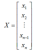
Before going into the mathematical definition for general case, let's start with specific cases first. Let's assum that we have a single column data as shown below.
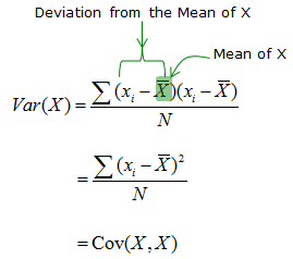
Variance of the data X can be defined as follows : (As you see, in case of single column data, Variance is same as covariance between the same data).
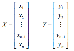
Now let's assume that we have two set of single column data as shown below.
If we calculate the variance of each data set separately, it would be as follows.
The covariance between these two data set (two single column data) is defined as follows :
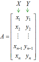
If you combine the two sets of data into a matrix form as shown below
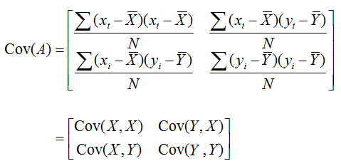
The covariance comes out as a matrix as shown below. (Since it has 2 columns of data, the covariance matrix becomes 2 x 2 matrix)
If the average of each data set (each column) is zero, the covariance matrix of the matrix can be calculated as follows. (AWGN (Additive White Gaussian Noise) is a good example of this kind of data)
Properties of Covariance Matrix
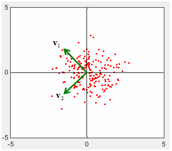
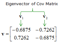
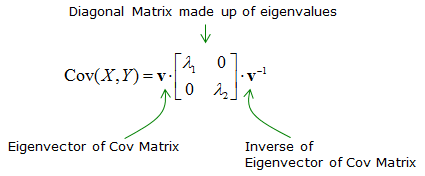
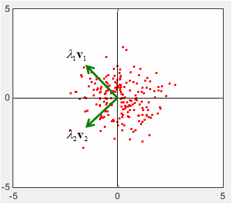
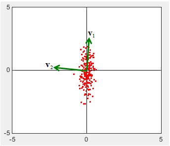
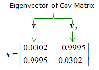
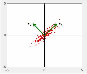
Graphical Implication of Covariance Matrix
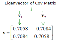
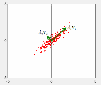
X = 0.25*randn(1,200); Y = randn(1,200); A = [cos(pi/4) sin(pi/4);-sin(pi/4) cos(pi/4)]; Tx = A * [X;Y]; X = Tx(1,:); Y = Tx(2,:); c=cov(X,Y) plot(X,Y,'ro','MarkerFaceColor',[1 0 0],'MarkerSize',2.0); axis([-5 5 -5 5]); [v,l]=eigs(c) v * l * inv(v)
Covariation vs. Correlation
Why Covariance Matrix ?
In most cases, Covariance matrix is applied to a long sequence of data set (i.e, multiple huge vectors) but it is not easy to get any useful information directly from the original data itself (we don't have much mathematical tools for it). But taking the covariance matrix from those dataset, we can get a lot of useful information with various mathematical tools that are already developed. This is possible mainly because of the following properties of covariance matrix.
|
||
