The degree matrix is the simplest of the graph matrices, because it keeps only one number per vertex. It does not tell you which vertices are connected. It only tells you how many edges each vertex has. That sounds like too little to be useful, but the degree matrix appears in almost every formula that combines it with the adjacency matrix, starting with the Laplacian. I'll give the definition first, then work one example, and then show where the matrix is used.

• Definition
• Example
• Directed and Weighted Graphs
• Where the Degree Matrix Is Used

Definition

Degree matrix is a diagonal matrix in which each diagonal elements indicate the degree of each vertex. (Formal defintion is as follows). It is written for an undirected graph without edge weights. The section on directed and weighted graphs further down shows how the definition changes for those cases.

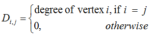
For a graph with n vertices, D is an n x n matrix. The element D_i,i is deg(v_i), the number of edges that touch v_i. Every element off the diagonal is 0. A common short form is D = diag(d₁, d₂, ..., d_n), where d_i = deg(v_i).

You can also get D from the adjacency matrix A in one step. The degree of v_i is the sum of row i of A, because each 1 in that row is one edge from v_i. So D = diag(A1), where 1 is the vector of all ones. One detail needs care. A loop at v_i counts 2 toward deg(v_i), because both ends of the loop touch v_i. The row sum of A only gives this when the loop is entered as 2 in a_ii.

• D is always diagonal : It holds the degrees on the diagonal and 0 everywhere else.
• D comes from the row sums of A : d_i is the sum of row i of the adjacency matrix.
• D alone does not define the graph : Many different graphs share the same degree list, so D is almost always used together with A.

Example

For example, let's assume that we have a graph as shown below. The graph has five vertices and six edges: v1-v2, v2-v3, v2-v4, v2-v5, v3-v4 and v4-v5. Count the lines at each vertex before you look at the matrix after it.

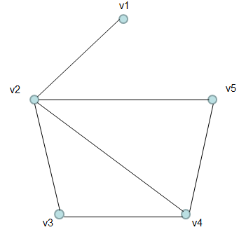
The Degree Matrix for this graph is as follows : (Try to generate this matrix on your own based on the definition of Degree of a vertex)

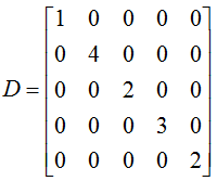
The diagonal reads 1, 4, 2, 3 and 2. v1 has only the edge to v2, so its degree is 1. v2 is joined to all four other vertices, so its degree is 4. The trace of D is 1 + 4 + 2 + 3 + 2 = 12, which is twice the six edges. This is the handshaking lemma in matrix form: trace(D) = 2|E|. Each edge adds 1 to the degree of each of its two ends, so the sum is always even.

The same numbers appear in two other places. They are the row sums of the adjacency matrix of this graph. They are also the diagonal of A², because a walk of length 2 from v_i back to v_i goes out along one edge and back along the same edge. This graph is used again on the Laplacian Matrix page.

• The degrees of this graph are 1, 4, 2, 3 and 2 : v2 is the most connected vertex and v1 the least.
• trace(D) = 2|E| : Here 12 = 2 x 6.
• diag(A²) = diag(D) for a simple graph : Each edge gives one closed walk of length 2 from each of its ends.

Directed and Weighted Graphs

The definition above assumes an undirected graph without weights. Both extensions change what "degree" means, so the degree matrix changes with them. Check which version a formula uses before you apply it.

In a directed graph, each vertex has an out-degree and an in-degree. So there are two degree matrices. D_out holds the number of edges that leave each vertex, and D_in holds the number that arrive. With the convention a_ij = 1 for an edge from v_i to v_j, D_out comes from the row sums of A and D_in from the column sums. For the directed example on the adjacency matrix page, D_out = diag(1, 0, 1, 2) and D_in = diag(1, 1, 2, 0). Both traces are 4, the number of edges.

In a weighted graph, the degree of v_i is the sum of the weights of its edges, d_i = w_i1 + w_i2 + ... + w_in. This is still the row sum of the weighted adjacency matrix W. Some texts call it the strength of the vertex. When every weight is 1, it is the ordinary degree again.

• A directed graph needs two degree matrices : D_out from the row sums of A, and D_in from the column sums.
• A weighted degree is a sum of weights : d_i is the row sum of W, and it does not have to be an integer.
• The diagonal form stays the same : Only the numbers on the diagonal change.

Where the Degree Matrix Is Used

On its own, D carries little information. Its value comes from what happens when you combine it with A. The combinations below are the ones you will meet most often.

The first is the Laplacian, L = D - A. For the example graph, the eigenvalues of L are 0, 1, 2, 4 and 5. The Laplacian Matrix page works through it. The second is the normalized Laplacian, D^-1/2 L D^-1/2. It needs D^-1/2, so every degree has to be positive. A graph with an isolated vertex has a 0 on the diagonal of D, and texts treat that vertex as a special case. The third is the random walk matrix, P = D^-1A. A walker at v_i moves to each neighbor with probability 1/d_i. For the example graph, the row of P for v2 is 0.25 for each of v1, v3, v4 and v5, and every row of P sums to 1.

One special case is worth noting. When every vertex has the same degree k, the graph is called k-regular, and D = kI. Then L = kI - A, so the eigenvalues of L are k minus the eigenvalues of A. For a regular graph, the Laplacian and the adjacency matrix give the same information.

• L = D - A is the main use : The Laplacian of the example graph has the eigenvalues 0, 1, 2, 4 and 5.
• Normalization needs positive degrees : D^-1/2 and D^-1 do not exist when a vertex has degree 0.
• D^-1A is a probability matrix : Each row sums to 1, which describes a random walk on the graph.
• A k-regular graph has D = kI : Its Laplacian eigenvalues are k minus its adjacency eigenvalues.