In this page, I will briefly describe on the list of terminologies that are commonly used in Graph Theory. I will explain directly on this page about the simple concept, but I will write a separate pages that would require long/detailed explanation.

• Vertex and Edge
• Degree
• Size
• Path and Cycle
• Hamiltonion Path/Cycle
• Eulerian Cycle/Circuit
• Distance
• Adjacency Matrix
• Incidence Matrix

Vertex and Edge

In the realm of graph theory, two fundamental concepts are indispensable: vertices and edges. Vertices, also known as nodes, represent discrete entities or points, which can symbolize various real-world elements such as cities, people, or data points. Edges, the connections between these vertices, denote the relationships or interactions between these entities. This framework of vertices connected by edges allows for the modeling and analysis of networks in many fields, including computer science, biology, and social science, providing valuable insights into the structure and dynamics of complex systems.

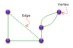
• Vertex (Vertices): In graph theory, a vertex (or node) is a fundamental unit from which graphs are formed. In the above diagram, each purple circle represents a vertex. Vertices can be used to represent objects, locations, or entities in various applications.
• Edge: An edge is a line connecting two vertices in a graph. It represents a relationship or connection between the vertices. In the above diagram, the green lines are edges. Edges can be undirected (no directionality) or directed (having a direction), though the ones in the above diagram are undirected.

A graph is usually written as G = (V, E). V is the set of vertices, and E is the set of edges. Each edge is written by the pair of vertices it joins, for example (u, v). In an undirected graph, (u, v) and (v, u) are the same edge. In a directed graph, the edge has a direction and goes from u to v only, so the two pairs are different edges.

Look at the two curved edges on the right of the diagram. They join the same pair of vertices. Two edges like that are called parallel edges, or multiple edges. An edge that starts and ends at the same vertex is called a loop. A graph with neither parallel edges nor loops is a simple graph, and a graph that allows parallel edges is often called a multigraph. So the graph in the diagram is a multigraph. The Konigsberg bridge graph on the What is Graph page is a multigraph for the same reason.

• A graph is two sets : the vertex set V and the edge set E. Every other term on this page is defined from these two sets.
• Direction is part of the edge : in a directed graph, an arrow from u to v does not allow travel from v to u.
• Check for parallel edges and loops : many formulas on this page assume a simple graph, so check this before you use them.

Degree 

The degree of a vertex in graph theory is a fundamental metric that quantifies the number of edges incident to a vertex, essentially measuring its connectivity within the graph. This concept plays a pivotal role in understanding the structure and behavior of networks, providing insights into the complexity and robustness of the networked system. Whether in analyzing social networks, optimizing transportation routes, or designing efficient communication systems, the degree of a vertex serves as a key analytical tool in numerous applications.

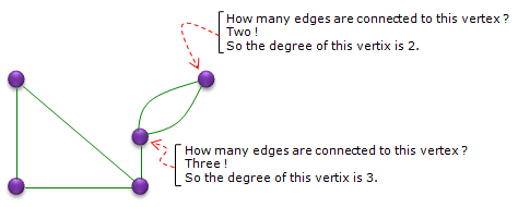
• Degree of a Vertex: The degree of a vertex in a graph is defined as the number of edges connected to that vertex. It quantifies the immediate connectivity of a vertex within the graph.

Let's add up the degrees of all five vertices in the diagram. The two vertices on the left have degree 2. The bottom right vertex and the middle vertex have degree 3. The top right vertex has degree 2. The total is 2 + 2 + 3 + 3 + 2 = 12. The graph has 6 edges, and 12 is exactly 2 x 6.

This is not a coincidence. Each edge has two ends, and each end adds 1 to the degree of one vertex. So the sum of all degrees is always twice the number of edges. This rule is called the handshake lemma. It has a useful consequence: the number of vertices with an odd degree is always even. The Eulerian Cycle/Circuit section below uses odd and even degrees directly.

In a directed graph, one number is not enough. The in-degree of a vertex counts the edges that arrive at it, and the out-degree counts the edges that leave it. The sum of all in-degrees and the sum of all out-degrees are both equal to the number of edges.

• Sum of degrees = 2 x number of edges : you can use this to check an edge count, or to find the number of edges from a degree list.
• Odd degree vertices come in pairs : a graph can never have exactly one vertex, or exactly three vertices, with an odd degree.
• A loop adds 2 to the degree : both ends of a loop sit on the same vertex, so the handshake lemma still holds.

Size

This size of a graph is a basic yet crucial characteristic that describes how many edges are present in a graph. The size of a graph is instrumental in understanding its complexity and the potential for connections among nodes, affecting both the theoretical properties and practical applications of the graph in various domains such as network analysis, algorithm design, and computational biology.

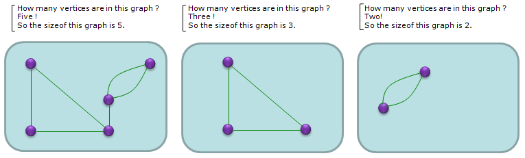
Be careful with the word size, because the diagram above and most textbooks use it differently. The diagram counts vertices and calls that number the size. In most graph theory textbooks, the number of vertices |V| is called the order of the graph, and the number of edges |E| is called the size. The table below gives both numbers for the three graphs in the diagram.

The two numbers are linked for a simple graph. Each edge joins a different pair of vertices, so a simple graph with n vertices has at most n(n - 1)/2 edges. For example, a simple graph of order 5 has a size of at most 10. The left and right graphs in the diagram are not simple, because each has two parallel curved edges.

• Order counts vertices, size counts edges : this is the textbook convention, and algorithm costs are usually written with both, for example O(|V| + |E|).
• Check the convention of your source : when a text says size, confirm whether it counts vertices or edges before you use the number.

Path and Cycle

In graph theory, understanding the structure and relationships within a network often revolves around two key concepts: paths and cycles. A path in a graph is defined as a sequence of vertices connected by edges where each vertex is visited exactly once, except possibly the first and last vertices. This structure is crucial for problems involving traversal, routing, and connectivity. On the other hand, a cycle represents a path whose starting and ending vertices are the same, creating a loop. Cycles are particularly significant because they can indicate redundancy in networks, circulation in flow systems, or feedback loops in circuit designs. Together, paths and cycles form the backbone of many algorithms and are essential for analyzing and interpreting the behavior of complex networks.

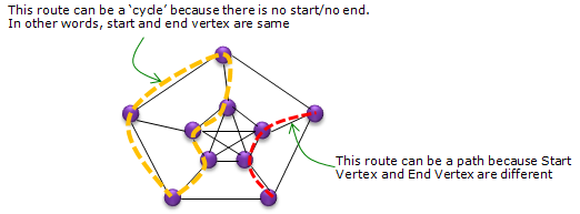
• Path: A path in a graph is a sequence of edges that connects a sequence of distinct vertices, where no vertex is visited more than once. In the above graph, the route highlighted with the red dashed line represents a path. It begins at one vertex and ends at another distinct vertex, without repeating any vertices along the route. This path is used to demonstrate a simple journey from a starting point to an endpoint, which is common in scenarios like routing and navigation.
• Cycle: A cycle is a path in which the start vertex and end vertex are the same, forming a closed loop. This means that the path returns to its original starting point. In the above graph, the cycle is indicated by the yellow dashed line. The cycle covers multiple vertices and returns to the starting vertex, creating a loop. This concept is crucial in applications like network design and circuit testing, where returning to the starting point without revisiting any other vertex is necessary.

Hamiltonion Path/Cycle

A Hamiltonian path in a graph is a path that visits each vertex exactly once. If this path returns to the starting vertex, forming a closed loop, it is called a Hamiltonian cycle. These constructs are important for understanding complex connectivity and routing problems, such as in logistics or network design, where each point (or vertex) needs to be visited precisely once.

These Hamiltonian paths and cycles are vital for solving problems where you must visit every point or node once without repetition, like in certain puzzles, scheduling tasks, or even the famous "Traveling Salesman Problem" in optimization discussions. Understanding these concepts can provide deep insights into the complexity and tractability of network routing challenges.

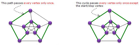
• Hamiltonian Path:
• The Hamiltonian path connects all the vertices in the graph without revisiting any. This path does not close back on itself, meaning it starts and ends at different vertices.
• In the graph above, the path is marked with green edges that connect all the purple vertices exactly once without forming a loop.
• Hamiltonian Cycle:
• The Hamiltonian cycle also visits each vertex exactly once but differs from the path by returning to the starting vertex, thus forming a loop.
• In the graph above, This cycle is depicted with green edges that form a closed circuit, returning to the initial vertex after traversing all other vertices exactly once.

Eulerian Cycle/Circuit 

An Eulerian cycle, or Eulerian circuit, is a cycle in a graph which visits every edge exactly once. This cycle starts and ends at the same vertex, encompassing all edges without repeating any. Eulerian cycles are a key concept in the study of graph theory and are particularly significant in solving real-world problems that involve traversing paths in an efficient manner, such as in the routing of garbage collection vehicles in cities or in postman routes where each road needs to be traveled exactly once.

Understanding Eulerian cycles is crucial for designing efficient algorithms in network routing and circuit design, ensuring minimal travel or movement while covering all necessary connections. This concept also helps in understanding the feasibility of constructing such paths or cycles in given graphs based on their structure and edge connectivity.

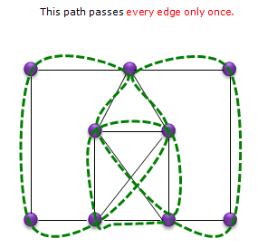
Euler found a simple test for this in 1736, when he solved the Konigsberg bridge problem. A connected graph has an Eulerian circuit exactly when every vertex has an even degree. The reason is that the circuit enters and leaves each vertex the same number of times. So the edges at each vertex are used in pairs, and the degree must be even.

A slightly weaker question asks for an Eulerian path, which uses every edge once but may end at a different vertex. A connected graph has an Eulerian path exactly when it has zero or two vertices of odd degree. With two, the path must start at one of them and end at the other. The Konigsberg graph has four vertices of odd degree, 5, 3, 3 and 3, so it has neither an Eulerian circuit nor an Eulerian path.

• Eulerian means every edge once : Hamiltonian means every vertex once. The two names are easy to mix up.
• The Eulerian test is easy : you only count degrees. The Hamiltonian question has no known test of this kind, and deciding it for a general graph is NP-complete.

Distance

In graph theory, the distance between two vertices is defined as the minimum number of edges that must be traversed to travel from one vertex to the other. This metric is crucial for understanding the efficiency of connectivity within a network and is often used in applications such as routing, navigation, and network design. The shortest path represents the most direct route between the two points, minimizing the cost, time, or distance traveled.

For example, there are many different paths connecting the vertices A and B. But the number of edges on path 1 are used to calculate the distance because it goes through the least number of edges between A and B. The distance between A and B is 2 in this example.

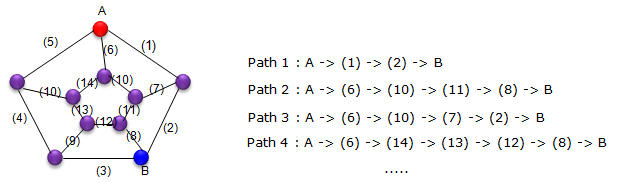
How does a computer find this distance in a large graph ? For an unweighted graph, it uses breadth first search. It starts at A, marks all neighbors of A as distance 1, then all their unmarked neighbors as distance 2, and so on until it reaches B. In the diagram, B is reached in the second round, so the distance is 2.

In many networks the edges are not equal. A link can have a delay or a cost, so each edge carries a weight. The distance is then the smallest total weight of a path, not the smallest number of edges. Dijkstra's algorithm finds it when all weights are non-negative. Link state routing protocols such as OSPF use this algorithm to compute the shortest path from each router to every other router.

• Distance uses the shortest path only : Path 2, Path 3 and Path 4 in the diagram also connect A and B, but they do not change the distance.
• Unweighted means breadth first search : each round of the search adds one edge to the distance.
• Weighted means Dijkstra : the same idea, but the search always expands the vertex with the smallest total weight so far.