A linear differential equation often has to be solved again and again with a different right-hand side. The Green function lets you do the hard work once. You solve the equation for a single impulse, and every other right-hand side then becomes an integral. I'll first state the definition and show why it gives the solution. Then we'll work through the operator minus second derivative and solve a few equations with it. The last sections show the matrix view and the places where engineers meet the same idea under other names.

• What is a Green function ?
• Why is the Green function useful ?
• Example
• How do you solve an equation with the example Green function ?
• What does the Green function look like as a matrix ?
• Where do engineers meet the Green function ?

What is a Green function ?

Before the definition, recall the delta function δ(x - a). It is zero everywhere except at x = a, and its integral is 1. So it models a unit impulse placed at one point, such as a point load on a beam or a point charge in space.

Green Function is a special function which is for a specific operator. It is a function that satisfy the following specific condition. It is named after a British mathematician George Green, who first developed the concept in the 1820s. This is widely used for linear partial differential equation.

The condition below says that the operator L, applied to G(x, a) as a function of x, gives a delta function at x = a. In words, G(x, a) is the response at x to a unit impulse placed at a.

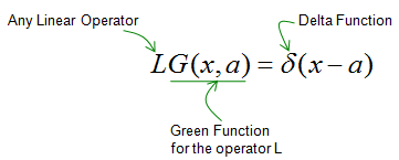
Figure 1. The defining condition of a Green function. The linear operator L turns G(x, a) into a unit impulse at x = a.

• G has two variables with different roles : x is where you observe the response, and a is where the impulse sits. L acts on x only.
• The operator must be linear : the whole method rests on adding the responses to many impulses. That sum is valid only when L is linear.
• Boundary conditions belong to G : the same operator has different Green functions on different domains or with different boundary conditions. G has to satisfy the boundary conditions of the problem you want to solve.
• Green published it in 1828 : the idea first appeared in his essay on electricity and magnetism, printed in 1828.

Why is the Green function useful ?

A formula for one impulse does not look like much at first. Its value appears when the same operator meets many different right-hand sides, such as many load patterns on one beam or many input signals to one circuit.

Then you may ask 'Why Green Function is important ?', 'Why we have to care about this ?'.

It is because this is very useful in some application especially when solving a differential equation.

Let's see the reason before the formulas. Any right-hand side f(x) can be written as a sum of impulses, one at every point a, each scaled by f(a). The Green function already gives the response to one impulse. So the response to f is the same sum of Green functions, and that sum is an integral.

For example, let's assume that we have a following equation.

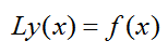
Figure 2. The equation to solve. L is the operator, f(x) is the known right-hand side, and y(x) is the unknown.

If we can derive a Green Function for this operator, you can have the solution for this equation just by applying following equation whatever the y(x) and f(x) is.

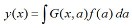
Figure 3. The solution formula. The solution is a weighted sum of impulse responses, with the weight f(a) at each point a.

• The proof is one line : apply L to both sides. L passes inside the integral because it acts on x and not on a. So L y(x) = ∫ δ(x - a) f(a) da = f(x).
• f can be anything, but y cannot : the formula works for any right-hand side f(x). The unknown y(x) is what the formula produces, so the phrase "whatever the y(x)" means that no guess about y is needed.
• The integral runs over the domain of the problem : for a problem on 0 <= x <= 1, a also runs from 0 to 1.
• The work is done once : finding G is the hard part. After that, every new f(x) costs only one integral.

Example

The simplest useful case is a string or a thin rod on 0 <= x <= 1, fixed at both ends so that G(0, a) = G(1, a) = 0. Its operator is minus the second derivative, and its Green function can be drawn with two straight lines.

One example for Green Function is as follows. In this case, the operator is '- second derivative'.

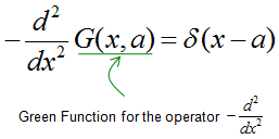
Figure 4. The condition for the operator minus d²/dx². The second derivative of G must be zero everywhere except at x = a.

A function that can satisfy the above condition is as follows.

The plot below draws G(x, a) as a function of x for one fixed a. It rises in a straight line from 0 at the left end, peaks at x = a, and falls in a straight line back to 0 at the right end.

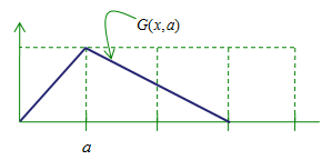
Figure 5. The Green function of minus d²/dx² with fixed ends. It is a triangle with a corner at the impulse point a.

How do you know if this function can meet the differential equation (solution for the differential equation). See here.

• The formula has two pieces : on 0 <= x <= 1 with fixed ends, G(x, a) = x(1 - a) for x <= a. To the right of the peak, G(x, a) = a(1 - x) for x >= a. The peak height at x = a is a(1 - a).
• Straight lines have a zero second derivative : so minus G'' is 0 everywhere except at the corner, which matches the delta function away from x = a.
• The corner carries the impulse : the slope is 1 - a on the left and -a on the right. It drops by exactly 1 at x = a, so minus G'' is a delta function of weight 1.
• G is symmetric : G(x, a) = G(a, x). The response at x to an impulse at a equals the response at a to an impulse at x.

How do you solve an equation with the example Green function ?

Now let's use the triangle to solve real equations. The problem is -y''(x) = f(x) on 0 <= x <= 1 with y(0) = y(1) = 0. Because G has two pieces, the integral from Figure 3 splits at a = x into two parts.

For a < x the impulse point lies left of x, so the second piece a(1 - x) applies. For a > x the first piece x(1 - a) applies. The solution is therefore y(x) = (1 - x) ∫₀^x a f(a) da + x ∫_x¹ (1 - a) f(a) da.

• The constant load gives a parabola : for f = 1 the two integrals are (1 - x) x²/2 and x (1 - x)²/2. Their sum is x(1 - x)/2.
• The boundary conditions hold automatically : every G(x, a) is zero at x = 0 and x = 1, so every sum of them is zero there too. You never fit integration constants.
• The sine row is an eigenfunction : sin(πx) comes back scaled by 1/π², because minus its second derivative is π² sin(πx).
• All three rows were checked : differentiating each y(x) twice returns the f(x) in its row.

What does the Green function look like as a matrix ?

On a computer, the operator becomes a matrix and the equation becomes a linear system. So it is natural to ask where the Green function goes. The answer is short: it becomes the inverse matrix.

Take N equally spaced interior points x_i = i h with h = 1/(N + 1). The second difference replaces minus the second derivative, so the operator becomes the matrix K = (1/h²) tridiag(-1, 2, -1). The equation -y'' = f becomes K y = f, and the solution is y = K^-1 f.

Compare that with y(x) = ∫ G(x, a) f(a) da. A sum with step h replaces the integral, so K^-1 should be close to h G(x_i, x_j). For this operator it is exact. With N = 4, h = 0.2, the grid is 0.2, 0.4, 0.6, 0.8, and K^-1/h equals the table below entry by entry.

• Each column is a sampled triangle : the column for x_j = 0.4 reads 0.12, 0.24, 0.16, 0.08. It peaks at 0.24 = 0.4 x 0.6, which is the peak height a(1 - a) of Figure 5.
• The matrix is symmetric : this is the discrete form of G(x, a) = G(a, x).
• The constant load checks out : K^-1 times a vector of ones gives 0.08, 0.12, 0.12, 0.08. These are exactly x(1 - x)/2 at the four grid points.
• A Green function is an inverse : the operator L plays the role of K, and G plays the role of K^-1. That is why G exists only when L y = 0 has no nonzero solution under the boundary conditions, just as K^-1 needs K to be invertible.

Where do engineers meet the Green function ?

Many engineers use Green functions every day without the name. Whenever a linear system is described by its response to an impulse, that response is a Green function. The fields below use the same idea with their own vocabulary.

The most common case is a linear time-invariant system. Its operator does not change with time, so the response to an impulse at time τ depends only on the delay t - τ. The Green function then reduces to the impulse response, G(t, τ) = h(t - τ). The formula of Figure 3 becomes y(t) = ∫ h(t - τ) f(τ) dτ, which is the convolution y = h * f from signals and systems.

The same structure appears in space as well as in time. In electrostatics, the operator is minus the Laplacian in three dimensions, and its Green function in free space is 1/(4π |r - r'|). This is the potential of a unit point charge, up to the constant ε₀. The potential of any charge distribution is then the integral of that point response over the charge.

• Impulse response and Green function are the same object : an LTI system turns G(t, τ) into h(t - τ), and the Green integral into a convolution.
• A wireless channel is described the same way : the channel impulse response is the Green function of the propagation environment, and the received signal is the transmitted signal convolved with it.
• Point sources explain the physics : a point load on a string, a point charge and a unit impulse on a circuit input all play the role of δ.
• The method requires linearity : a nonlinear system, such as an amplifier driven into saturation, has no single impulse response. The superposition behind Figure 3 then fails.