This page is to give you some intuitive understanding of meaning of several patterns of differential equations, not too much about the solution itself. In real life, you wouldn't find many of differential equation which can be solved intuitively as described in this page. But the way I describe in this page would give you more familiarity to various differential equations and I hope you can be less "scared" about differential equation.

However, I expect you to have some previous exposures to the concept of basic calculus like the concent of derivatives.

• y' = y
• y' = y, y(0) = 2
• -u'' = delta(x-1/3)

y' = y

The question behind this first pattern is simple: which function is its own derivative? Let's answer it by guessing and checking, without any solution method. The same guess-and-check idea is also the first step of many formal methods, so it is worth doing slowly once.

First pattern of differential equation I want to look into is as follows.

Now just try to vervalize the meaning of this equation based on what you learned in basic calculus course. I can describe it as follows.

i) There is a function called y(x)

ii) The first derivative of y(x) equals to itself (y(x)).

The only thing you have to do now is to make some GUESS on what kind of function has the characteristics as mentioned above. Actually it would not be easy to make a guess if you do not have any knowledge about calculus. But if you just look into well known tables like this, you may find a function that meets this requirement. It is the exponential function.

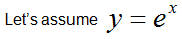
Then what is the first derivative of y ?

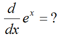
The answer is as follows. You see the function e^(x) satisfy the equation and property saying "The first derivative of y(x) equals to itself (y(x))". If you can find another function meeting the requirement, that can be the solution for this differential equation.. or if you can even create your own function whatever it is, that can be the solution too.

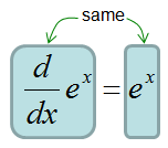
Is this the only function that satisfy the equation ?

Now let take another function and plug into the equation. I chose the function y(x) = 2 e^(x) in this case

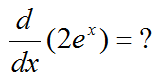
What is the answer ? It is as follows. From this, you see 2 e^(x) also meets the criteria of "The first derivative of y(x) equals to itself (y(x))". So 2 e^(x) can be a solution for the differential equation.

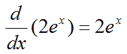
Now let's try to find some other functions. As you see in the following example, you would find the infinite number of functions that can be the solution to the differential equation given in this example.

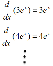
Based on all the functions that we found above, you can come out with a general form of equation as follows.

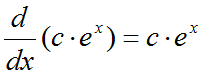
According to the equation above, you can say a generic function shown below meets the differential equation. This is called a general solution for the equation.

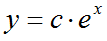
Let's check that c e^x covers every solution, and not only the ones we happened to guess. Suppose y(x) is any solution of y' = y. Look at the product y(x)e^-x. Its derivative is y'e^-x - ye^-x = (y' - y)e^-x = 0. A function with zero derivative everywhere is a constant, so y(x)e^-x = c, and y(x) = ce^x. So the general solution really is complete. The constant c can be any real number, and c = 0 gives the zero function, which is also a solution.

The same guess works for a small change of the equation. For y' = ky, try y = ce^kx. Its derivative is kce^kx = ky, so it fits for every c. A positive k gives growth, as in population or compound interest. A negative k gives decay, as in cooling or radioactive decay. This one family covers a large share of the first order models you meet in engineering.

• A differential equation has a family of solutions : y' = y is satisfied by every function ce^x, one for each value of c.
• The family is complete : The product ye^-x has zero derivative, so no solution exists outside ce^x.
• One free constant for a first order equation : The single constant c is what an extra condition, such as an initial value, will fix.

y' = y, y(0) = 2

In previous example, you could find a solution to a differential equation based on the intuitive interpretation of the equation itself and simple derivative table. One problem was we had too many solution to the equation. It is not because our method is wrong, but because we have not enough information to pick any one specific function as the solution.  

Now let's look at another differential equation as shown below. The first part is exactly same as in the previous example. The only difference is that we have one additional information (This kind of additional information is a boundary condition or boundary value. or in this example case, it is called 'initial value' or 'initial condition' because it gives only a single condition at the starting point)

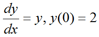
As we did in previous example, let's verbalize this equation. (let's describe the equation in plain language). It is as described below.

i) There is a function called y(x)

ii) The first derivative of y(x) equals to itself (y(x)).

iii) There is one condition saying "y(0) should be 2". It means the value of the function y(x) at the point x = 0 is 2.

The way you can find solution for this kind is equation is

a) Find all the possible solution to a give differential equation

b) Plug the additional information into the all the candidate solution, and pick a specific function that meets the boundary condition.

We already did step a) in previous example.. so I would not redo this step.

Now let's do step b). If you plug the initial condition (y(0) == 2) into the all the candidate function (general solution) that we got from step a), only one function meets the give initial condition as shown below. So y(x) = 2 e^x is the solution for the differential equation in this example.

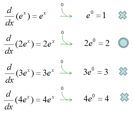
Checking the candidates one by one works here, but it does not scale. Let's use the general solution directly instead. Put x = 0 into y = ce^x. Because e⁰ = 1, you get y(0) = c. The initial condition y(0) = 2 then gives c = 2 in one step, without testing c = 1, 3, 4 and so on. The same step works for any initial value y₀. The solution of y' = ky with y(0) = y₀ is y = y₀e^kx.

Notice that one condition was enough here. The equation is first order, so its general solution has exactly one free constant, and one condition fixes it. A second order equation has two free constants, and it needs two conditions. The next example has two, u(0) = 0 and u(1) = 0. They are given at the two ends of an interval, so they are called boundary conditions rather than initial conditions.

• Solve for the constant, do not search for it : Substitute the condition into the general solution, here c e⁰ = 2, so c = 2.
• The number of conditions matches the order : A first order equation needs one condition, and a second order equation needs two.
• Initial value versus boundary value : Conditions given at one starting point are initial conditions. Conditions given at two ends are boundary conditions.

-u'' = delta(x-1/3)

This example would not be as intuitive as previous example and you would not found the solution from the tables in a calculus book. But I put this as an example since it can greatly help you with the concept of 'Green Function'.

Let's suppose we have a second order differential equation as shown below. At first part we have a differential equation and in second, the third we have boundary conditions.

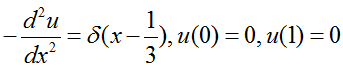
Just a little modification, we can rewrite the equation as follows. You don't have to do this, but I did this form matches better with the graphical representation that we will go through.

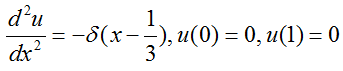
How can we find the solution to this equation ? Unfortunately it is not that straightforward and I would not explain it in this page now. In stead, let's just suppose that we are given a function and check if the given function meets the given differential equation.

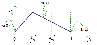
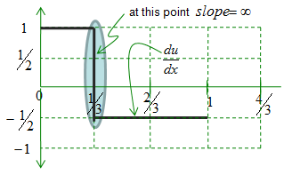
Now let's take the first derivative of this function. It is easy.. it is like figuring out the slope of a graph that you learned in high school physics and math. If you plot the first derivative (u'(x)) in a graph, you would get a plot as shown below. (Note that it looks like a step function).

Now let take another derivative of the above graph. Since this is derivative of the first derivative, it became the second derivative of the original function. The graph looks as follows and now you can realize that the second derivative of the given function (u''(x)) matches the given differential equation.

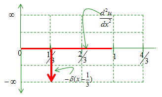
Let's check the numbers on the graphs above, because they do not quite match the equation. The graph of u(x) rises to 1/3 at x = 1/3 and falls back to 0 at x = 1. So its slope is 1 on the left and -1/2 on the right, and the u'(x) graph shows exactly these two values. The slope therefore jumps by -3/2 at x = 1/3. But the equation -u'' = δ(x - 1/3) asks for a jump of exactly -1. Here is the reason. Integrate u'' = -δ(x - 1/3) over a small interval around x = 1/3, and the change of u' across that point is -1. So the function drawn above solves -u'' = (3/2)δ(x - 1/3). Its shape is right, and its height is 3/2 times too large.

We can find the correct function with the same picture in mind. Away from x = 1/3 the equation says u'' = 0, so u is a straight line on each side. The condition u(0) = 0 gives u = Ax on the left. The condition u(1) = 0 gives u = B(1 - x) on the right. The two lines must meet at x = 1/3, so A/3 = 2B/3, or A = 2B. The slope must jump by -1, so -B - A = -1. Together these give A = 2/3 and B = 1/3. So u(x) = 2x/3 for x ≤ 1/3 and u(x) = (1 - x)/3 for x ≥ 1/3. The peak is u(1/3) = 2/9, not 1/3.

The same steps work for a point load at any position a between 0 and 1. The result is u(x) = x(1 - a) for x ≤ a and u(x) = a(1 - x) for x ≥ a. This function of x and a is the Green function of -u'' with these two boundary conditions. Physically, it is the shape of a tight string fixed at both ends and pushed by a unit point force at x = a.

• Between the point loads the solution is a straight line : u'' = 0 there, so each piece has a constant slope.
• A delta function makes a kink : -u'' = δ(x - a) makes the slope u' drop by exactly 1 at x = a, while u itself stays continuous.
• The boundary conditions and the jump fix the answer : For a = 1/3 they give the slopes 2/3 and -1/3, and the peak value 2/9.
• This is the Green function : Its general form is x(1 - a) for x ≤ a and a(1 - x) for x ≥ a.