My own image for a matrix is a kind of machine that is doing things as follows. As you see in the illustration, Matrix is taking in a shape (geometrical shape/object) and transform (change shape) them in mainly three different way as follows.

i) Scale (magnify or shrink)

ii) Rotate

iii) Skew

In reality, a matrix can do more than one type of transformation like "Scale and Skew", "Scale and Rotate and Skew" etc.

I will talk about this kind of transformation in this section and I hope you can have some intuitive understanding of the propery of a matrix since it can be visualized as in this section.

Figure 1. A matrix as a transformation machine. A square goes in, and it comes out scaled, rotated, sheared, or changed by any combination of the three.

• Expand/Contract : the label in the drawing for what the text above calls Scale. The square changes size.
• Rotate : the square turns around the origin without changing size or shape.
• Shear : the label for Skew. The square leans into a parallelogram.
• The output pile at the bottom : shows shapes made by combining the three steps, which is what a general matrix does.

I will write this note at two different angles.

The first angle keeps the grid fixed and moves the shape. The second angle keeps the numbers of each point fixed and moves the grid. Both angles describe the same matrix, and the second section shows why they always give the same final picture.

• Matrix as a Shape Transformer
• Matrix as a Coordinate System Transformer

Matrix as a Shape Transformer

I think one of the best way to understand the characteristics of a Matrix is to apply it for an shape in a graphical coordinates and observe the result. Of course, there would be a certain limitation in this method since we can only visualize three dimensional shape and as a result the dimension of the matrix we can visualize would be 3 x 3 (or 4 x 4 in some cases). But if you build up a solid intuitive understanding of a properties of a matrix in this way, you can easily extend the understanding to any size of the matrix and, more importantly, you can understand more easily a mathematical model represented in the matrix format.

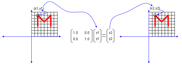
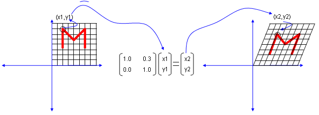
I will use a shape in two dimensional coordinate and 2 x 2 matrix applying to the shape on the coordinate. Here you see coordinates labeled (x1,y1) and (x2,y2). (x1,y1) represents each points before it is transformed by the matrix and (x2,y2) is the new points after (x1,y1) is transformed by the matrix.

Let's look at the first case. The first matrix is what we call Identity Matrix which has the value '1' in all the elements on diagonal line running from left top to right bottom and all the other elements are set to be '0'.

What is the result of the transformation of a shape transformed by the Identity Matrix ? The answer is "No change".

Figure 2. The identity matrix. Every point (x1,y1) is mapped to itself, so the M does not move.

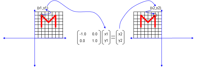
Next look at another matrix shown below. This matrix also looks similar to Identity Matrix but not exactly same. The difference is that the first element on the diagonal line is '-1' in stead of '1'.  What is the result ?

The shape is flipped around y axis.

Figure 3. The matrix with -1 and 1 on the diagonal. It maps (x1,y1) to (-x1,y1), which flips the shape around the y axis.

The right plot of Figure 3 does not show this flip. It still has the M in the first quadrant, as in Figure 2. With x2 = -x1, every point moves to the other side of the y axis, so the M should appear in the second quadrant. The M is symmetric, so its mirror image looks the same, but its position changes.

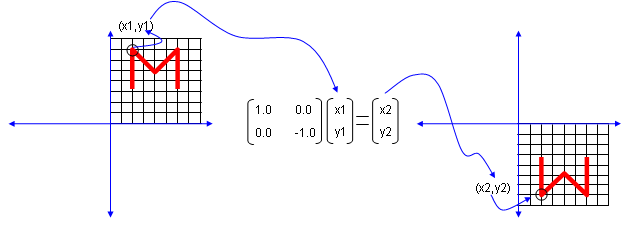
Next look at another matrix shown below. This matrix also looks similar to Identity Matrix but not exactly same. The difference is that the second element on the diagonal line is '-1' in stead of '1'.  What is the result ?

The shape is flipped around x axis.

Figure 4. The matrix with 1 and -1 on the diagonal. It maps (x1,y1) to (x1,-y1), so the M flips below the x axis and reads as a W.

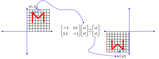
Next look at another matrix shown below. In this case, all the elements on the diagonal lines is set to be '-1' instead of '1'.  What is the result ?

It became reflected around the point (0,0). You can interpret this in two steps.

At the first step, the shape is flipped around y axis. and at the second step the shape is fliped around x axis.

Figure 5. The matrix with -1 and -1 on the diagonal. It maps (x1,y1) to (-x1,-y1), a reflection through the origin that moves the M into the third quadrant.

Now let's look at another matrix as shown below. This time you see all '1's on the diagonal line and now you see a non-zero value out side of diagonal line. What is the result ?

The image shears.

Figure 6. The shear matrix with 0.3 in the upper right. It maps (x1,y1) to (x1 + 0.3 y1, y1), so points move right in proportion to their height.

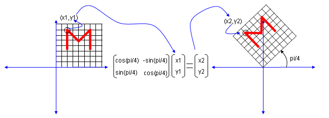
Now let's look at another matrix as shown below. This time you see the non-zero value in all the elements. This is tricky to analyze since these matrix can do almost everything described above.. but if the numbers in the elements can be represented as trigonometrix functions in the following format. This matrix can rotate the image as shown below.

Figure 7. The rotation matrix with cos(pi/4) and sin(pi/4). The M turns counterclockwise by π/4 around the origin, without any change of size or shape.

Actually this is only a few of the examples.. you can try any numbers in the matrix and apply to some shape and try to correlate those numbers to the result of the transformation until you build up your own intuition of figuring out the characteristics of a matrix.

Let's collect these matrices in one place and add one number to each: the determinant. Its absolute value is the factor by which the area of a shape changes. Its sign tells you whether the shape is mirrored. A negative determinant means the M comes out mirrored, as in the two single-axis flips.

Notice that the reflection through (0,0) has determinant 1, not -1. Two flips cancel each other's mirror effect. So the M is turned upside down, but it is not mirrored, and the same matrix is also a rotation by π. The shear and the rotation keep the area too, because their determinant is 1. A scale matrix such as [2, 0; 0, 2] doubles both sides of a shape and multiplies its area by 4, which is its determinant.

There is one more pattern in these examples. The first column of each matrix is where the point (1, 0) goes, and the second column is where (0, 1) goes. For the shear, (0, 1) goes to (0.3, 1), so the top of the grid leans right by 0.3. This column view is the starting point of the next section.

• Diagonal entries scale or flip one axis : a -1 on the diagonal flips that axis, and a value like 2 stretches it.
• Off-diagonal entries mix the axes : they produce the shear, and together with the diagonal they produce rotations.
• The determinant measures area and orientation : its size is the area factor, and a negative sign means a mirror image.
• Each column is the image of one basis vector : reading the columns tells you where the unit square goes.

Matrix as a Coordinate System Transformer

Now I will introduce you another way to interpret the meaning of a matrix in terms of transformation. If a matrix is given in a well known form (well known numbers) as shown in previous section, you may figure out the characteristics of the matrix right away. But you may find it difficult to figure out the meaning of the matrix if the numbers in the matrix is not so familiar to you.  What I am going to introduce in this section would help you understand the meaning of the matrix in any form of the matrix.

Let me explain with a specific example. Let's assume that we have a matrix as shown below.

Figure 8. The example matrix M. Its first column is (1, 0), and its second column is (-0.7071, 0.7071).

First, let's think of this matrix as a combination of two column vectors and represent the two column vectors in a coordinate system. I will show you two different way of representation of the column vectors as shown below.

In Interpretation (I), you have the two column vectors plotted as in the plot [B]. In this interpretation, you can say two basis vector shown in plot [A] is transformed to different coordinates (vectors) in Plot [B] which is represented by the column vectors of the matrix M. More specifically, the vector (0,1) is transformed to coordinate (-0.7071,0.7071) by the matrix M and the vector (1,0) is transformed to coordinate (1.0,0.0) by the matrix M.

In Interpretation (II), you see the same column vectors in plot [C]. But you would notice that the coordinates of the vectors (meaning the numbers in the vectors) are different from the one in plot [B]. The coordinate in plot [C] is same as in plot [A]. But you see the obvious differences of the two sets of vectors in the plot [A] and plot [C]. How can the different looking vectors can have the same coordinate (coordinate value) ? If you look at the plots a little bit more carefully, you would notice that the coordinate system (grid lines) in plot [C] is different from plot [A]. In this case, we can interpret that the matrix transforms the whole coordinate system and each individual coordinate (the coordinate of individual vectors) stays same in the new (transformed) coordinate. In this specific example, you can say the vector (0,1) in original coordinate system (plot [A])  is mapped to the same coordinate (0,1) in the new (transformed) coordinate in plot [C] and the vector (1,0) in original coordinate system (plot [A])  is mapped to the same coordinate (1,0) in the new (transformed) coordinate in plot [C]

NOTE : Click here or on the image, it will lead you to slide show pages and you would get more intuitive understandings.

Figure 9. Two interpretations of the same matrix M. In Interpretation (I), the vectors move on a fixed grid. In Interpretation (II), the grid moves, and the coordinates stay (1, 0) and (0, 1).

• Plot [A] : the original grid with the basis vectors (1, 0) in red and (0, 1) in blue.
• Plot [B] : the same grid with the two column vectors of M drawn on it. The blue vector now points up and to the left.
• Plot [C] : a slanted grid built from the column vectors of M. On this grid, the red and blue vectors still have the coordinates (1, 0) and (0, 1).

For more intutive understandings, I put some more examples as shown below. Click on the images for the full slideshow pages.

Figure 10. Both basis vectors change direction and length. In plot [C], the new grid lines are no longer perpendicular.

Figure 11. Both basis vectors turn by the same angle and keep their length. The new grid in plot [C] is the original square grid, rotated as a whole.

Figure 12 and the two figures below it switch from single vectors to a block of points. Each quarter of the block has its own color, so you can follow each quarter through the transformation.

Figure 12. A block of colored points under a matrix that turns only the second basis vector. The squares become parallelograms, and plots [B] and [C] show the same result.

Figure 13. The same block under a matrix that turns and scales both basis vectors. The squares become thin rhombi.

Figure 14. The same block under a pure rotation. The four colored squares keep their shape and turn together.

Let's follow one point through both interpretations of M, the matrix of Figure 8. Take the point with coordinates (1, 1). In Interpretation (I), M moves it on the original grid to M(1, 1) = (1 - 0.7071, 0.7071) = (0.2929, 0.7071). In Interpretation (II), the point keeps its coordinates (1, 1), but you read them on the new grid. One step along the first new axis and one step along the second new axis end at the same place, (0.2929, 0.7071) on the original grid. So the two interpretations always agree on where the point ends up. They differ only in the grid you use to read its numbers.

The inverse matrix translates in the other direction. For this M, M^-1 = [1, 1; 0, 1.4142]. A point at (1, 1) on the original grid has the coordinates M^-1(1, 1) = (2, 1.4142) on the new grid. The determinant of M is 0.7071, so each cell of the new grid has 0.7071 times the area of an original cell. A matrix with determinant 0 has no inverse, because its new grid collapses onto a line.

• The columns of M are the new axes : in Interpretation (II), they are the basis vectors of the transformed grid.
• Moving the points and moving the grid give the same picture : the final position of every point is M times its coordinates in both views.
• M^-1 converts back : it gives the coordinates of an original point on the new grid.
• A rotation keeps the grid square : Figure 11 and Figure 14 show a grid that turns without stretching, which is why their squares keep their shape.