In simple description, the Orthogonal Matrix is a special form of matrix in which each of the column vectors or row vectors are orthogonal to each other. (You may ask what is 'Orthogonal' ? The, refer to Orthogonality Page).

Orthogonal matrices appear everywhere in engineering math. A rotation is one, the Q of a QR decomposition is one, and the U and V of an SVD are two more. The reason is simple: their inverse needs no calculation, because it is just the transpose. I'll first list the properties that define the matrix, then test three examples against them. After that we'll look at what an orthogonal matrix does to a vector, and how to check one numerically.

• What properties define an orthogonal matrix ?
• Which of the three example matrices are orthogonal ?
• What does an orthogonal matrix do to a vector ?
• How do you check orthogonality in practice ?

What properties define an orthogonal matrix ?

The informal description above needs one more condition before it becomes a definition. Orthogonal columns alone are not enough, because each column must also have a length of 1. The two equations below state both conditions at once, in the form you'll use in a calculation.

If I list up the properties of Orthogonal Matrix in more details, it is as follows

• It is a Square Matrix
• Each of the column vectors or row vectors are orthogonal to each other, and each of them has a length of 1
• Following equation are always met (Inner product of a Matrix and its transpose produce an Identity Matrix)

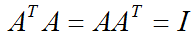
Figure 1. The defining equation. The product of the matrix and its transpose, in either order, is the identity matrix.

• Following equation are always met (Transpose of the matrix is same as the inverse of the matrix.)

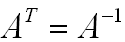
Figure 2. The same property stated as an inverse. The transpose of an orthogonal matrix is its inverse.

Let's see why Figure 1 contains both conditions. Write a₁, a₂, ..., a_n for the columns of A. The entry in row i and column j of A^TA is the inner product a_i^Ta_j. For this product to be the identity matrix, every off-diagonal entry must be 0 and every diagonal entry must be 1. A zero off-diagonal entry means that two different columns are orthogonal. A diagonal entry of 1 means that a_i^Ta_i = 1, so each column has a length of 1. Columns with both properties are called orthonormal.

The same argument applied to AA^T gives the rows. For a square matrix, A^TA = I already forces AA^T = I, so orthonormal columns and orthonormal rows always come together.

• Orthogonal columns are not enough : the matrix D = diag(2, 3) has orthogonal columns, but D^TD = diag(4, 9), which is not I. So D is not an orthogonal matrix.
• The name does not say orthonormal : an orthogonal matrix has orthonormal columns. There is no separate name for a matrix whose columns are only orthogonal.
• Figure 2 follows from Figure 1 : A^TA = I says that A^T undoes A, which is the definition of A^-1.
• The complex version is the unitary matrix : for complex entries, the conjugate transpose replaces the transpose, and the condition becomes U^HU = I. See Unitary Matrix.

Which of the three example matrices are orthogonal ?

Each example below applies Figure 2 directly. The transpose is computed from the matrix on the left, the inverse is computed separately, and the two results are compared. If they match, the matrix is orthogonal.

A couple of examples would give you better understanding. Is following matrix (the matrix in the left). Yes it is because its transpose and inverse are same.

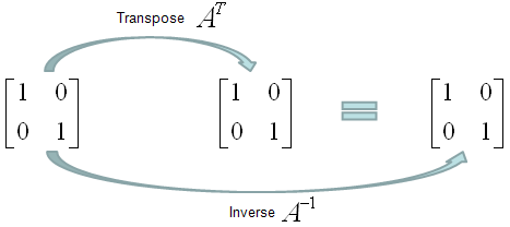
Figure 3. The identity matrix. Its transpose and its inverse are both the identity matrix, so it is orthogonal.

• Left : A = [[1, 0], [0, 1]], where each inner bracket is one row.
• Upper arrow : the transpose A^T is the same identity matrix.
• Lower arrow : the inverse A^-1 is also the identity matrix, and the two are equal.

Is following matrix (the matrix in the left) orthogonal. Yes it is because its transpose and inverse are same.

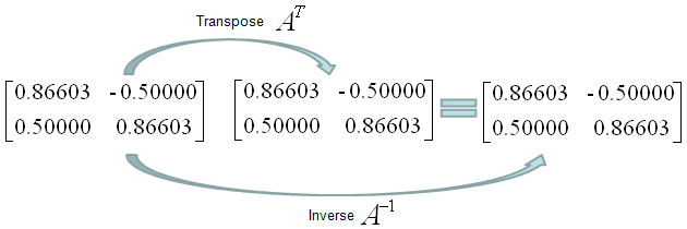
Figure 4. A rotation by 30 deg. The matrix is orthogonal, but the middle and right matrices in the picture repeat the original matrix instead of showing its transpose.

The matrix on the left is [[0.86603, -0.5], [0.5, 0.86603]]. The entries are cos 30 deg = 0.86603 and sin 30 deg = 0.5, so this is the rotation by 30 deg. The conclusion of the example is correct, and the matrix is orthogonal. But the two matrices in the middle and on the right are drawn wrong. Both repeat the original matrix. The transpose moves -0.5 to the lower left, so A^T = [[0.86603, 0.5], [-0.5, 0.86603]]. The inverse A^-1 is exactly the same matrix. It is the rotation by -30 deg, which undoes the first rotation.

• Column lengths : 0.86603² + 0.5² = 0.75 + 0.25 = 1 for both columns.
• Column inner product : 0.86603 x (-0.5) + 0.5 x 0.86603 = 0, so the two columns are orthogonal.
• Result : A^TA = I, and A^T = A^-1 = [[0.86603, 0.5], [-0.5, 0.86603]].

Is following matrix (the matrix in the left) orthogonal. No it is not because its transpose and inverse are not same.

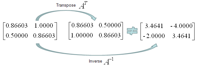
Figure 5. A matrix that is not orthogonal. Its transpose and its inverse are different matrices.

• Left : A = [[0.86603, 1.0], [0.5, 0.86603]]. Only the upper right entry differs from the rotation in Figure 4.
• Upper arrow : A^T = [[0.86603, 0.5], [1.0, 0.86603]], which is correct.
• Lower arrow : A^-1 = [[3.4641, -4.0], [-2.0, 3.4641]], which is also correct. The determinant is 0.86603² - 1.0 x 0.5 = 0.25, so every entry of the inverse is 4 times the matching adjugate entry.
• Why it fails : the second column [1.0, 0.86603] has a length of about 1.32, not 1. The inner product of the two columns is 0.86603 + 0.43301, about 1.30, not 0. So A^TA = [[1, 1.299], [1.299, 1.75]], which is far from I.

What does an orthogonal matrix do to a vector ?

The algebraic condition A^TA = I has a direct geometric meaning. An orthogonal matrix can turn or mirror a vector, but it cannot stretch it. This is why rotations and reflections are the typical examples.

Take any vector x and let y = Ax. The squared length of y is y^Ty = x^TA^TAx = x^Tx. So y has the same length as x. The same calculation with two vectors shows that the inner product is also kept, which means that the angle between two vectors does not change. For example, the rotation in Figure 4 maps x = [3, 4]^T to [0.598, 4.964]^T. Both vectors have length 5. The non-orthogonal matrix in Figure 5 maps the same x to [6.598, 4.964]^T, whose length is about 8.26.

The determinant gives the second geometric fact. From A^TA = I, det(A)² = 1, so det(A) is either +1 or -1. A determinant of +1 means a rotation. The rotation in Figure 4 has det(A) = 1. A determinant of -1 means a reflection, possibly combined with a rotation. For example, [[1, 0], [0, -1]] mirrors a vector at the horizontal axis, and its determinant is -1.

• Length and angle are preserved : |Ax| = |x| and (Ax)^T(Ay) = x^Ty for every x and y.
• The determinant is +1 or -1 : +1 for a rotation and -1 for a reflection. See Determinant.
• Every eigenvalue has magnitude 1 : the rotation by 30 deg has the complex eigenvalues 0.86603 + 0.5j and 0.86603 - 0.5j, and both have magnitude 1.
• Products stay orthogonal : if A and B are orthogonal, then (AB)^T(AB) = B^TA^TAB = I. Two rotations in a row are again a rotation.

How do you check orthogonality in practice ?

The examples above compare the transpose with the inverse. That works, but it needs a matrix inversion, and it compares two full matrices by eye. In practice, it is simpler to compute A^TA and compare it with the identity matrix.

With real numbers, the comparison must allow a small tolerance. The entries 0.86603 and 0.5 in Figure 4 are rounded, and a computer stores cos 30 deg only to about 16 digits. So the computed A^TA is close to I, but not exactly equal. The listing below shows the check in Matlab and in Python.

% Matlab / Octave
A   = [cosd(30) -sind(30); sind(30) cosd(30)];
err = norm(A'*A - eye(2));      % close to 0 for an orthogonal matrix
isOrth = err < 1e-12;

# Python / numpy
import numpy as np
c, s = np.cos(np.pi/6), np.sin(np.pi/6)
A = np.array([[c, -s], [s, c]])
print(np.allclose(A.T @ A, np.eye(2)))   # True

Once a matrix is known to be orthogonal, you can use the property to save work. A system Ax = b is solved by x = A^Tb, with no elimination at all. This is also numerically safe, because multiplying by an orthogonal matrix does not amplify rounding errors. That is one reason why the QR decomposition and the SVD are built from orthogonal matrices.

• Test A^TA against I : this one product checks the orthogonality and the unit length of all columns at once.
• Use a tolerance : floating point values never give an exact identity matrix, so compare with a small threshold.
• Solve with the transpose : for an orthogonal A, x = A^Tb solves Ax = b, and the condition number of A is exactly 1.
• Related pages : see QR Decomposition and SVD for decompositions that produce orthogonal matrices.