Before you multiply two vectors or two matrices, you have to check whether the product exists at all. The check uses only the sizes of the two factors. It also tells you the size of the result before you compute a single entry. This page shows the size rule first and then applies it to six examples. The first three multiply two vectors of three elements, and the last three multiply two 2 x 3 matrices. Each example tries a different combination of transposes, so you can see which combinations work and what shape each one gives.

• What is the size rule for a product ?
• What happens when two vectors are multiplied ?
• What happens when two 2 x 3 matrices are multiplied ?
• What do the six examples give with real numbers ?

What is the size rule for a product ?

Every entry of a matrix product pairs one row of the left factor with one column of the right factor. The pairing works only if the row and the column have the same number of elements. That single requirement is the whole size rule.

The diagram below writes the left factor as m x n and the right factor as a x b. The two inner numbers, n and a, must be equal. The two outer numbers, m and b, give the size of the result.

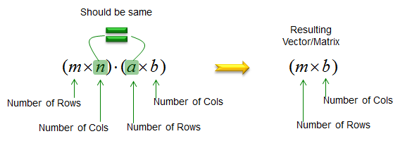
Figure 1. The size rule. The number of columns of the left factor must equal the number of rows of the right factor, and the result is m x b.

• Should be same : n is the number of columns of the left factor, and a is the number of rows of the right factor. The product exists only when n = a.
• Resulting Vector/Matrix : the result has m rows, taken from the left factor, and b columns, taken from the right factor.
• The shared size disappears : n = a is the length of each row-column pair. It is summed over, so it does not appear in the size of the result.
• Order matters : a 2 x 3 matrix times a 3 x 2 matrix gives 2 x 2, but the same two matrices in the other order give 3 x 3.

The same rule covers a matrix times a vector. An m x n matrix times an n x 1 column vector gives an m x 1 column vector. A 1 x m row vector times an m x n matrix gives a 1 x n row vector. For a chain of products, you apply the rule pair by pair. For example, (2 x 3)(3 x 4)(4 x 1) gives 2 x 4 after the first step and 2 x 1 after the second.

The sizes also give the cost of a product. The result has m x b entries, and each entry needs n multiplications. So the product needs m x n x b multiplications. In a chain, the order of evaluation changes this count, although it never changes the result. Take A as 10 x 100, B as 100 x 5 and C as 5 x 50. Computing (AB)C costs 10 x 100 x 5 + 10 x 5 x 50 = 7500 multiplications. Computing A(BC) costs 100 x 5 x 50 + 10 x 100 x 50 = 75000, ten times more.

What happens when two vectors are multiplied ?

A vector is a matrix with a single row or a single column. So the size rule applies to vectors without any change. The three examples below use the same two row vectors, v₁ and v₂, each with three elements. They differ only in where the transpose goes.

Example 1 >

First, let's try to multiply the two row vectors as they are. Figure 2 defines the vectors, Figure 3 asks for the product, and Figure 4 applies the size rule.

Figure 2. The two row vectors. The last element of v₂ is printed as a₃₃, which is a typo for a₂₃.

Figure 3. The question. Can a row vector multiply another row vector ?

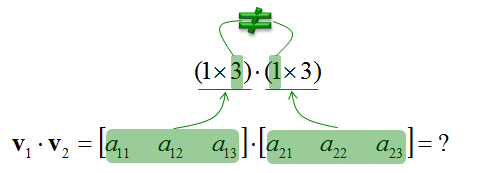
Figure 4. The size check fails. The inner numbers are 3 and 1, so v₁ x v₂ is not defined.

• The typo in Figure 2 : v₂ = [a₂₁ a₂₂ a₂₃], as Figures 3 and 4 show. The a₃₃ in Figure 2 is a typo.
• Why it fails : v₁ has 3 columns, but v₂ has only 1 row. Each row of v₁ would need a column of 3 elements to pair with, and v₂ has no such column.
• The dot is not the dot product here : on this page the dot means the matrix product. The dot product of two vectors is the product written in Example 2.

Example 2 >

Now transpose the second vector. The column vector v₂^T has 3 rows, which matches the 3 columns of v₁.

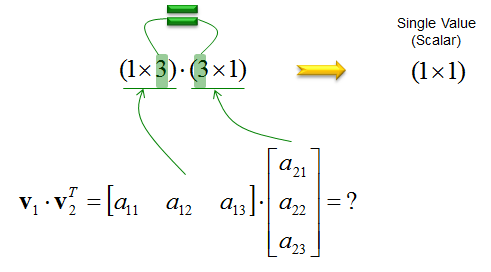
Figure 5. The size check passes. A 1 x 3 row times a 3 x 1 column gives a 1 x 1 result, a single value.

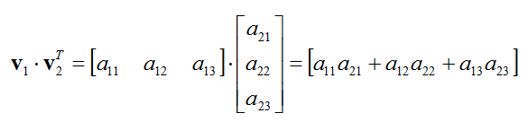
Figure 6. The result. The single entry is the sum of the three element-by-element products.

• This is the inner product : v₁v₂^T = a₁₁a₂₁ + a₁₂a₂₂ + a₁₃a₂₃. It is the dot product of the two vectors, written as a matrix product. See Inner Product.
• The result is written in brackets : the picture shows the 1 x 1 result as a matrix with one entry. In practice it is treated as a scalar.
• A zero result means orthogonal vectors : if the sum is 0, the two vectors are orthogonal.

Example 3>

Finally, move the transpose to the first vector. The column v₁^T has only one column, so it needs a right factor with one row. The row vector v₂ has exactly that. Figure 7 repeats the question of Example 2, v₁v₂^T. Figures 8 and 9 show the actual question, v₁^Tv₂.

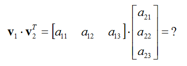
Figure 7. The question of Example 2, v₁v₂^T, shown again. It does not match the product computed in this example.

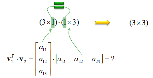
Figure 8. The size check passes. A 3 x 1 column times a 1 x 3 row gives a 3 x 3 matrix.

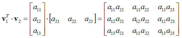
Figure 9. The result. Every element of v₁ multiplies every element of v₂.

• This is the outer product : the entry in row i and column j is a_1ia_2j. The shared size is 1, so each entry is a single product and no sum is needed.
• Same vectors, very different results : Example 2 gives one number, and this example gives nine. The only change is the position of the transpose.
• The outer product has rank 1 : every row of the result is a multiple of v₂. Its diagonal entries add up to the inner product of Example 2.

What happens when two 2 x 3 matrices are multiplied ?

The same three experiments work with matrices. The difference is that each factor now has two rows, so the result has more entries. The examples below use m₁ and m₂, two 2 x 3 matrices, and again move the transpose from nowhere, to the second factor, to the first factor.

Example 4>

First, let's try m₁m₂ with no transpose. Figure 10 defines the two matrices, and Figures 11 and 12 repeat the steps of Example 1.

Figure 10. The two matrices. Both m₁ and m₂ are 2 x 3.

Figure 11. The question. Can one 2 x 3 matrix multiply another 2 x 3 matrix ?

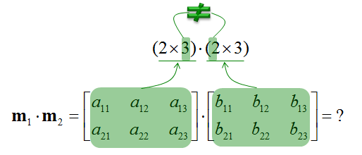
Figure 12. The size check fails. The inner numbers are 3 and 2, so m₁m₂ is not defined.

• Same shape is not enough : two matrices of the same size can always be added, but they can be multiplied only if they are square.
• Why it fails : each row of m₁ has 3 elements, while each column of m₂ has only 2.

Example 5>

Now transpose the second factor. The transpose m₂^T is 3 x 2, so its 3 rows match the 3 columns of m₁.

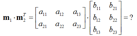
Figure 13. The question. The transpose turns the rows of m₂ into columns.

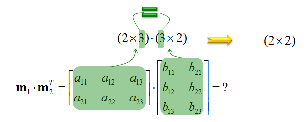
Figure 14. The size check passes. A 2 x 3 matrix times a 3 x 2 matrix gives a 2 x 2 matrix.

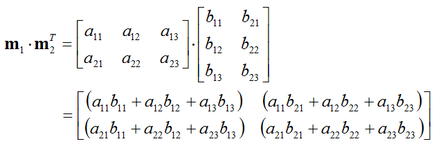
Figure 15. The result. Each entry is the inner product of one row of m₁ and one row of m₂.

• Top left : a₁₁b₁₁ + a₁₂b₁₂ + a₁₃b₁₃, the inner product of row 1 of m₁ and row 1 of m₂.
• Top right : a₁₁b₂₁ + a₁₂b₂₂ + a₁₃b₂₃, row 1 of m₁ with row 2 of m₂.
• Bottom row : the same two sums with row 2 of m₁. So entry (i, j) is row i of m₁ times row j of m₂.
• This is Example 2 repeated four times : each entry is one inner product of the kind computed in Example 2.

Example 6>

Finally, transpose the first factor. The transpose m₁^T is 3 x 2, and its 2 columns match the 2 rows of m₂.

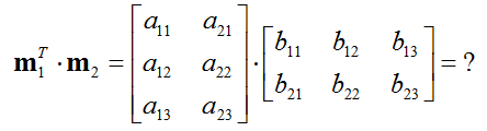
Figure 16. The question. The transpose turns the rows of m₁ into columns.

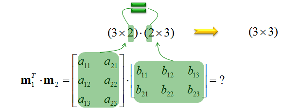
Figure 17. The size check passes. A 3 x 2 matrix times a 2 x 3 matrix gives a 3 x 3 matrix.

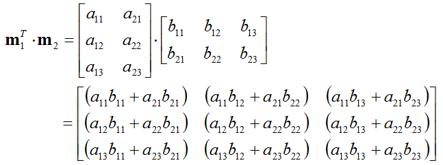
Figure 18. The result. Each entry is a sum of only two products, because the shared size is 2.

• Entry (i, j) : a_1ib_1j + a_2ib_2j, which is column i of m₁ times column j of m₂.
• A sum of two outer products : the result equals the outer product of row 1 of m₁ and row 1 of m₂, plus the same for row 2. Each term has the shape of Example 3.
• The rank is at most 2 : the 3 x 3 result is built from two rank-one terms, so it can never have rank 3.

What do the six examples give with real numbers ?

The symbolic results above are easier to trust after a numeric check. So let's put small integers into the same six products and compare the sizes with the size rule. Take v₁ = [1, 2, 3], v₂ = [4, 5, 6], m₁ = [[1, 2, 3], [4, 5, 6]] and m₂ = [[1, 0, 2], [0, 1, 1]], where each inner bracket is one row.

Example 1   v1 * v2       1 x 3 times 1 x 3   not defined
Example 2   v1 * v2^T     1 x 3 times 3 x 1   = 1*4 + 2*5 + 3*6 = 32
Example 3   v1^T * v2     3 x 1 times 1 x 3   = [  4   5   6 ]
                                                [  8  10  12 ]
                                                [ 12  15  18 ]
Example 4   m1 * m2       2 x 3 times 2 x 3   not defined
Example 5   m1 * m2^T     2 x 3 times 3 x 2   = [  7   5 ]
                                                [ 16  11 ]
Example 6   m1^T * m2     3 x 2 times 2 x 3   = [  1   4   6 ]
                                                [  2   5   9 ]
                                                [  3   6  12 ]

The numbers confirm the observations above. The diagonal of the Example 3 result is 4, 10 and 18, and its sum is 32, the inner product of Example 2. The Example 6 result has rank 2, and its diagonal sum, 18, equals the diagonal sum of the Example 5 result, 7 + 11. That is the identity trace(AB) = trace(BA) with A = m₁^T and B = m₂.

In software, the matrix product and the element-wise product use different operators. In Matlab, v1*v2' is the matrix product of Example 2, and m1.*m2 multiplies entry by entry. In numpy, the matrix product is written v1 @ v2.T and the element-wise product is m1 * m2. The element-wise product needs two factors of the same size, so for m₁ and m₂ it exists even though the matrix product of Example 4 does not. It gives [[1, 0, 6], [0, 5, 6]].

• Check the inner numbers first : (m x n)(n x b) gives m x b. Examples 1 and 4 fail this check, and the other four pass it.
• The transpose decides the shape : the same data give a scalar, a 3 x 3 matrix, a 2 x 2 matrix or no result at all, depending only on where the transpose goes.
• Row times column means inner product : every entry of a defined product is a sum over the shared size. When the shared size is 1, the sum has one term, and the product is an outer product.
• More on the product : the Multiplication page traces each entry of a 2 x 2 product, and the Dimension page lists the size rule for more shapes.