QR Decomposition is a method of splitting a matrix into multiplication of following two matrix. Q has orthonormal columns, and R is an upper triangular matrix. The split works for any matrix whose columns are linearly independent, square or tall. It is the standard way to solve least squares problems on a computer.

• What do Q and R contain ?
• How do you calculate Q and R ?
• What is QR decomposition used for ?

What do Q and R contain ?

Before computing anything, let's see what the two factors hold. Both are built from the columns of A. Q keeps their directions and throws away their lengths, and R records how much of each column points along each direction of Q.

What does each of the matrix mean ? Each of the matrix in the equation indicates as shown below. As you see here, Q is made up of Orthogonal Unit Vectors and R is a Upper Triangular Matrix.

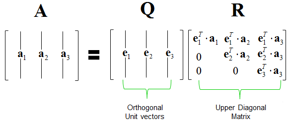
• R is upper triangular : the label under R in the picture says "Upper Diagonal Matrix". The correct name is upper triangular matrix, as the text above says. Every entry below the diagonal is 0.
• Each entry of R is a dot product : r_ij = e_i^T a_j, which is the length of a_j along e_i. Because Q^TQ is the identity matrix, the whole matrix is R = Q^TA.
• Why the lower part is zero : Gram Schmidt builds e₁, ..., e_j from a₁, ..., a_j only. So a_j lies in the span of the first j unit vectors, and it is orthogonal to every e_i with i > j.
• A column needs only the earlier e vectors : a₂ = r₁₂ e₁ + r₂₂ e₂, and a₃ needs e₁, e₂ and e₃. That is exactly the triangular shape of R.

How do you calculate Q and R ?

How do you calculate this ? If you look at the contents of Q and R, you will notice.. once you get Q matrix R can be derivated mechanically from the column vectors of A and element and the column vectors of Q. So the only thing you have to consider is how to derive Q matrix.

Q can be derived from A by a special method called Gram Schmidt Process. However, Gram Schmidt Process will derive an Orthogonal matrix but it is not guaranteed that all the vectors in the orthogonalized matrix. To make each of the vectors in the orthogonalized matrix, you just need to normalize each of the column vector of orthogonalized matrix produced by Gram Schmidt Process.

Now do you know what do you have to do ?  Yes, study Gram Schmidt Process :)

Let's run the process on a 3 x 3 example, so that you can check each number by hand. The columns of A are a₁ = (1, 1, 0), a₂ = (1, 0, 1) and a₃ = (0, 1, 1). In each step, we subtract the parts that point along the unit vectors we already have. Then we normalize what is left.

A = [ 1  1  0 ; 1  0  1 ; 0  1  1 ]

step 1   u1 = a1                              = ( 1, 1, 0 )                  |u1| = 1.4142
         e1 = u1 / |u1|                        = ( 0.7071, 0.7071, 0 )

step 2   r12 = e1T a2 = 0.7071
         u2 = a2 - r12 e1                    = ( 0.5, -0.5, 1 )             |u2| = 1.2247
         e2 = u2 / |u2|                        = ( 0.4082, -0.4082, 0.8165 )

step 3   r13 = e1T a3 = 0.7071      r23 = e2T a3 = 0.4082
         u3 = a3 - r13 e1 - r23 e2           = ( -0.6667, 0.6667, 0.6667 )  |u3| = 1.1547
         e3 = u3 / |u3|                        = ( -0.5774, 0.5774, 0.5774 )

Q = [ 0.7071  0.4082 -0.5774 ; 0.7071 -0.4082  0.5774 ; 0  0.8165  0.5774 ]
R = [ 1.4142  0.7071  0.7071 ; 0  1.2247  0.4082 ; 0  0  1.1547 ]

The diagonal of R holds the lengths |u₁|, |u₂| and |u₃|, so it is always positive in this process. The entries above the diagonal are the projections r_ij that step 2 and step 3 subtracted. If you multiply Q by R, you get A back, and Q^TQ is the identity matrix.

A library routine can give a different sign pattern. For example, numpy.linalg.qr uses Householder reflections, and for this A it returns the first column of Q and the first row of R with the opposite sign. Both answers are correct, because the two sign changes cancel in the product. So compare the product QR, not the individual entries, when you check a result.

• Gram Schmidt is the idea, not the best algorithm : the classical process loses orthogonality in floating point when the columns of A are nearly dependent. Numerical libraries use Householder reflections or modified Gram Schmidt instead.
• The columns must be independent : if a_j is a combination of the earlier columns, u_j is the zero vector and cannot be normalized. Then r_jj = 0, and A has no QR factorization with an invertible R.
• Signs are a convention : flipping the sign of column i of Q together with row i of R leaves the product unchanged. The factorization is unique only after you require a positive diagonal in R.

What is QR decomposition used for ?

So why would you factor a matrix into Q and R? Two uses dominate in practice. The first is least squares, where A is tall and Ax = b has no exact solution. The second is the QR algorithm, which is how software computes eigenvalues.

Let's start with least squares. We want the line y = x₁ + x₂ t through the points (0, 1), (1, 2), (2, 2) and (3, 4). Four points and two unknowns give a 4 x 2 system with no exact solution. With A = QR, the least squares solution comes from the small triangular system R x = Q^T b, solved by back substitution.

A = [ 1  0 ; 1  1 ; 1  2 ; 1  3 ]            b = [ 1 ; 2 ; 2 ; 4 ]

Q = [ 0.5 -0.6708 ; 0.5 -0.2236 ; 0.5  0.2236 ; 0.5  0.6708 ]
R = [ 2  3 ; 0  2.2361 ]                    QT b = [ 4.5 ; 2.0125 ]

R x = QT b   ->   x2 = 2.0125 / 2.2361 = 0.9
                  x1 = ( 4.5 - 3 x 0.9 ) / 2 = 0.9       so  y = 0.9 + 0.9 t

The normal equations A^TA x = A^Tb give the same answer here. But they square the condition number. For this A, the condition number is 3.76, and the condition number of A^TA is 14.13, which is 3.76². QR works on A directly, so it keeps the smaller number. For an ill-conditioned problem, that difference decides how many correct digits you get.

The QR algorithm uses the factorization in a loop. It factors A_k = Q_kR_k and then multiplies the factors in reverse order, A_k+1 = R_kQ_k. Since R_kQ_k = Q_k^TA_kQ_k, every A_k has the same eigenvalues as A. The off-diagonal entries shrink, and the diagonal converges to the eigenvalues. For A = [2 1 ; 1 2], whose eigenvalues are 3 and 1, the diagonal goes through the values below.

k        diagonal of Ak          |off-diagonal|
1        2.8000    1.2000         0.6000
2        2.9756    1.0244         0.2195
3        2.9973    1.0027         0.0740
4        2.9997    1.0003         0.0247

• QR is the safe way to do least squares : solving R x = Q^Tb avoids forming A^TA, so the condition number is not squared.
• The QR algorithm converges at a known rate : in the example, the off-diagonal entry shrinks by about 3 in each step, which is the ratio of the two eigenvalues, 3 / 1. Close eigenvalues make it slow, and practical versions add shifts to speed it up.
• Q preserves lengths : multiplying by Q^T does not change the norm of a vector. That is why errors do not grow when you move b into the coordinates of Q.