Every LTE cell sends the same short signal twice in each radio frame, and the UE looks for it first during cell search. The PSS gives the UE the OFDM symbol timing, the 5 ms half-frame timing and N_ID⁽²⁾, one of the two numbers that make up the physical cell ID.

PSS is a specific physical layer signal that is used for radio frame synchronization. It has characterstics as listed below.

• Mapped to 72 active sub carriers(6 resource blocks), centered around the DC subcarrier in slot 0 (Subframe 0) and slot 10 (Subframe 5) in FDD.
• Mapped to 72 active sub carriers(6 resource blocks), centered around the DC subcarrier in slot 2 (Subframe 1) and slot 12 (Subframe 6) in TDD.
• Made up of 62 Zadoff Chu Sequence Values
• Used for Downlink Frame Synchronization
• One of the critical factors determining Physical Cell ID

The physical cell ID is 3 N_ID⁽¹⁾ + N_ID⁽²⁾ (36.211 v19.3.0 clause 6.11). The PSS carries N_ID⁽²⁾, from 0 to 2, and the SSS carries N_ID⁽¹⁾, from 0 to 167, which gives 504 cell IDs. In TDD the PSS sits in the third OFDM symbol of subframes 1 and 6, three symbols after the SSS, while in FDD the two signals sit in adjacent symbols. A UE can use this gap to tell FDD from TDD.

This may not be an important topic for most of the case since it would be working fine for most of the device that you have for test. Otherwise it would have not been given to you for test.

However, If you are a developer working at early stage of LTE chipset, this would be one of the first signal you have to implement.

Followings are the topics to be covered in this page.

• Algorithm for PSS Generation
• Generating PSS with default Matlab function
• Cross Correlation between different PSS
• Correlation between a PSS and its PhaseShifted Version
• Correlation between a PSS and its Noised Version
• PSS detection in Action
• Frequeny Domain Correlation Method
• Time Domain Correlation Method
• Source Code in srsUE
• Frequency Adjustment with PSS
• Frequency Offset Estimation
• Frequency Offset Compensation
• Reference

Algorithm for PSS Generation

The exact PSS symbol calculation is done by the following formula as described in 36.211 - 6.11.1. For the specific example of generated PSS, refer to Matlab : Toolbox : LTE : PSS page or PSS with default Matlab function.

The diagram below has two parts. The upper part generates the 62 values d_u(n) from the root index u, and the lower part maps them to subcarriers around the centre of the carrier.

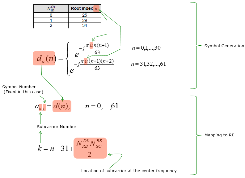
36.211 clause 6.11.1. The root index u comes from N_ID⁽²⁾, the two formulas generate d_u(n), and k places the 62 values around the centre subcarrier.

The sequence is a Zadoff-Chu sequence of length 63 with its middle element removed. The first formula covers n = 0 to 30, and the second covers n = 31 to 61 with the index shifted by one. So the element that would fall on the DC subcarrier is never generated. The mapping k = n - 31 + N_RB^DLN_sc^RB/2 then puts 31 values below and 31 values above the centre of the carrier.

36.211 v19.3.0 clause 6.11.1.2 also reserves 5 subcarriers on each side, for n = -5 to -1 and n = 62 to 66. So the PSS owns the central 72 subcarriers, 6 RB, at every bandwidth. That is why a UE can find the PSS before it knows the bandwidth of the cell.

The roots 29 and 34 add up to 63. A Zadoff-Chu root u and the root 63 - u give complex conjugate sequences, so the PSS for N_ID⁽²⁾ = 2 is the complex conjugate of the PSS for N_ID⁽²⁾ = 1. A receiver can use this to test both with one correlation.

• 62 values from a length-63 Zadoff-Chu sequence : the DC element is skipped.
• Central 72 subcarriers : 62 used and 5 reserved on each side, at every bandwidth.
• Roots 25, 29 and 34 : 29 and 34 are a conjugate pair.

Generating PSS with default Matlab function

The formula above is short enough to code directly, without the LTE Toolbox. The code below computes d_u(n) for one N_ID⁽²⁾, then plots the first half, the second half and the whole sequence.

Followings are the Matlab code for generating PSS and its result for each NID value.

clear all;

 

u_shift = [25 29 34];

 

NID = 0;

 

d_u = [];

 

for n = 0:61

    

    u = u_shift(NID+1);

    

    if n <= 30

        d = exp(-j*pi*u*n*(n+1)/63);    

    else

         d = exp(-j*pi*u*(n+1)*(n+2)/63);   

    end;

    

    d_u = [d_u d];

 

end;

 

subplot(1,3,1);

plot(real(d_u(1:31)),imag(d_u(1:31)),'ko','MarkerFaceColor',[0 0 0]);

axis([-1.5 1.5 -1.5 1.5]);

title('n=0..30');

 

subplot(1,3,2);

plot(real(d_u(32:62)),imag(d_u(32:62)),'bo','MarkerFaceColor',[0 0 1]);

axis([-1.5 1.5 -1.5 1.5]);

title('n=31..61');

 

subplot(1,3,3);

plot(real(d_u(1:62)),imag(d_u(1:62)),'ro','MarkerFaceColor',[1 0 0]);

axis([-1.5 1.5 -1.5 1.5]);

title('n=0..61');

 

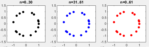
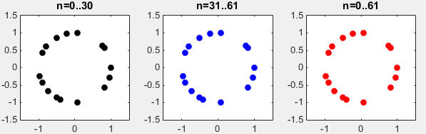
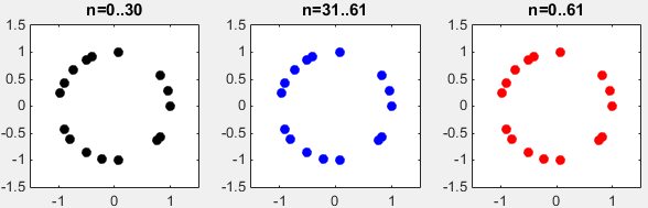
The 62 PSS values for N_ID⁽²⁾ = 0, 1 and 2, drawn as the first half, the second half and the whole sequence.

All 62 values lie on the unit circle, because each is a complex exponential. The two left plots in each row look identical. The PSS is symmetric, d_u(n) = d_u(61 - n), so the second half repeats the first half in reverse order and adds no new points. The rows for N_ID⁽²⁾ = 1 and 2 are mirror images about the real axis, because roots 29 and 34 are a conjugate pair.

Followings are the numberical result (print out of d_u[ ] array) for each NID;

The printout shows the same symmetry. The value at n = 0 is 1 for every root, and so is the value at n = 61.

• Constant amplitude : every value has magnitude 1.
• Symmetric sequence : d_u(n) = d_u(61 - n).
• N_ID⁽²⁾ = 1 and 2 mirror each other : complex conjugates.

Cross Correlation between different PSS

Threre are three types of PSSs in LTE. To make all these three type unique (distinctive to each other), it is designed that the cross correlation between each PSS be very low. Following example shows the cross correlation between each PSS.

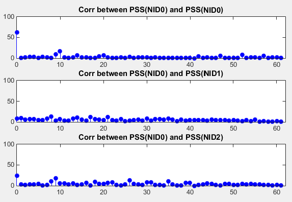
Correlation of the PSS for N_ID⁽²⁾ = 0 with itself and with the other two. Only the matching sequence gives a clear peak at lag 0.

Following is the Matlab source code that produce the result as shown above. I used Matlab dsp package to calculate the cross correlation. If you don't have Matlab dsp package, try to write your own script for calculating cross correlation

clear all;

 

u_shift = [25 29 34];

 

% Generate PSS for NID = 0

 

NID = 0;

d_u = [];

 

for n = 0:61

    

    u = u_shift(NID+1);

    

    if n <= 30

        d = exp(-j*pi*u*n*(n+1)/63);

    else

        d = exp(-j*pi*u*(n+1)*(n+2)/63);

    end;

    

    d_u = [d_u d];

 

end;

 

d_u_NID0 = d_u';

 

 

% Generate PSS for NID = 1

 

NID = 1;

d_u = [];

 

for n = 0:61

    

    u = u_shift(NID+1);

    

    if n <= 30

        d = exp(-j*pi*u*n*(n+1)/63);

    else

        d = exp(-j*pi*u*(n+1)*(n+2)/63);

    end;

    

    d_u = [d_u d];

 

end;

 

d_u_NID1 = d_u';

 

 

% Generate PSS for NID = 2

 

NID = 2;

d_u = [];

 

for n = 0:61

    

    u = u_shift(NID+1);

    

    if n <= 30

        d = exp(-j*pi*u*n*(n+1)/63);

    else

        d = exp(-j*pi*u*(n+1)*(n+2)/63);

    end;

    

    d_u = [d_u d];

 

end;

 

d_u_NID2 = d_u';

 

 

% Cross Correlation between PSS

 

Hxcorr = dsp.Crosscorrelator;

taps = 0:61;

taps = taps';

 

XCorr_0_0 = step(Hxcorr,d_u_NID0,d_u_NID0);

XCorr_0_1 = step(Hxcorr,d_u_NID0,d_u_NID1);

XCorr_0_2 = step(Hxcorr,d_u_NID0,d_u_NID2);

 

subplot(3,1,1);

stem(taps,abs(XCorr_0_0(62:end)),'bo','MarkerFaceColor',[0 0 1]);

xlim([0 length(taps)]); ylim([0 100]);

title('Corr between PSS(NID0) and PSS(NID0)');

 

subplot(3,1,2);

stem(taps,abs(XCorr_0_1(62:end)),'bo','MarkerFaceColor',[0 0 1]);

xlim([0 length(taps)]); ylim([0 100]);

title('Corr between PSS(NID0) and PSS(NID1)');

 

subplot(3,1,3);

stem(taps,abs(XCorr_0_2(62:end)),'bo','MarkerFaceColor',[0 0 1]);

xlim([0 length(taps)]); ylim([0 100]);

title('Corr between PSS(NID0) and PSS(NID2)');

 

 

The peaks in the plot can be checked by hand. At lag 0, a PSS correlated with itself gives 62, the number of values, because every product has magnitude 1. The same sum gives about 8 against the PSS for N_ID⁽²⁾ = 1 and about 24 against N_ID⁽²⁾ = 2. These match the values at lag 0 in the lower two plots, so the correct PSS stands out by a factor of more than 2.5 even against the closest root.

The code builds each column with d_u', which in Matlab is the conjugate transpose. The later examples use transpose() instead. Conjugating both inputs does not change the magnitude of a correlation, so the plots above are not affected.

• Self correlation 62 at lag 0 : the length of the sequence.
• About 8 and 24 against the other roots : at least 2.5 times smaller.
• d_u' conjugates : harmless for the magnitudes shown here.

Correlation between a PSS and its PhaseShifted Version

This example shows the correlation between a PSS and its phaseshifted copy. As you see here, the magnitue (absolute value) of correlation does not changes even if you do phase shift. However, you can figure out the degree of phase shift by taking the angle of correlation.

With this property, you can identify a PSS in a received signal without worrying about any possible phase shift that might have occurred by communication channel. In addition, you can figure out the amount of phase shift by taking the angle value of the correlation and use that value to compensate (undo) the phase shift.

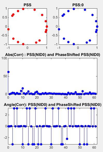
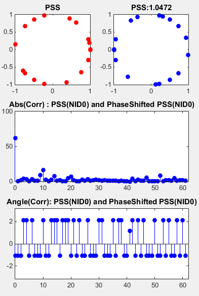
Left, the PSS correlated with an identical copy. Right, with a copy rotated by pi/3 rad. The magnitude is the same, and only the angle changes.

Following is the matlab source code that produced the result shown above. I used Matlab dsp package to calculate the cross correlation. If you don't have Matlab dsp package, try to write your own script for calculating cross correlation

clear all;

 

u_shift = [25 29 34];

 

% Generate PSS for NID = 0

 

NID = 0;

d_u = [];

 

for n = 0:61

    

    u = u_shift(NID+1);

    

    if n <= 30

        d = exp(-j*pi*u*n*(n+1)/63);

    else

        d = exp(-j*pi*u*(n+1)*(n+2)/63);

    end;

    

    d_u = [d_u d];

 

end;

 

phShift = pi/3;

d_u_NID0 = transpose(d_u); % Original PSS

d_u_NID0_PhaseShift = transpose(d_u .* exp(j*phShift)); % PhaseShifted PSS

 

 

% Cross Correlation between PSS

 

Hxcorr = dsp.Crosscorrelator;

taps = 0:61;

taps = taps';

 

XCorr_0_0_Shifted = step(Hxcorr,d_u_NID0,d_u_NID0_PhaseShift);

 

subplot(3,2,1);

plot(real(d_u_NID0),imag(d_u_NID0),'ro','MarkerFaceColor',[1 0 0]);

title('PSS');

 

subplot(3,2,2);

plot(real(d_u_NID0_PhaseShift),imag(d_u_NID0_PhaseShift),'bo','MarkerFaceColor',[0 0 1]);

title(strcat('PSS:',num2str(phShift)));

 

subplot(3,2,[3 4]);

stem(taps,abs(XCorr_0_0_Shifted(62:end)),'bo','MarkerFaceColor',[0 0 1]);

xlim([0 length(taps)]); ylim([0 100]);

title('Abs(Corr) : PSS(NID0) and PhaseShifted PSS(NID0)');

 

subplot(3,2,[5 6]);

stem(taps,angle(XCorr_0_0_Shifted(62:end)),'bo','MarkerFaceColor',[0 0 1]);

xlim([0 length(taps)]); ylim([-pi pi]);

title('Angle(Corr): PSS(NID0) and PhaseShifted PSS(NID0)');

In both plots the magnitude at lag 0 is 62, so a rotation of the whole sequence leaves the detection peak untouched. The angle at lag 0 is 0 for the identical copy and about -1.05 rad, which is -pi/3, for the rotated copy. The sign is negative because the correlator conjugates its second input. A receiver can therefore read the common phase rotation of the channel from the correlation peak.

• Magnitude unchanged by phase rotation : 62 at lag 0 in both cases.
• Angle at lag 0 = -pi/3 : the rotation, with the sign set by the conjugate.

Correlation between a PSS and its Noised Version

This example shows the noise tolerance of PSS. The example on the left shows the correlation between a PSS and the one with 50 dB SNR (practically no Noise condition) and the example on the right shows the correlation between a PSS and the one with 10 dB SNR.

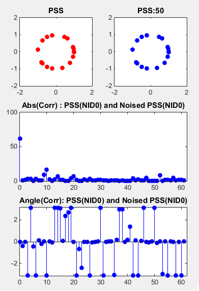
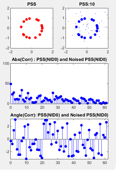
Left, SNR_dB = 50. Right, SNR_dB = 10. The peak at lag 0 survives the noise, but see the note below on the real SNR.

Following is the matlab source code that produced the result shown above. I used Matlab dsp package to calculate the cross correlation. If you don't have Matlab dsp package, try to write your own script for calculating cross correlation.

clear all;

 

u_shift = [25 29 34];

 

% Generate PSS for NID = 0

 

NID = 0;

d_u = [];

 

for n = 0:61

    

    u = u_shift(NID+1);

    

    if n <= 30

        d = exp(-j*pi*u*n*(n+1)/63);

    else

        d = exp(-j*pi*u*(n+1)*(n+2)/63);

    end;

    

    d_u = [d_u d];

 

end;

 

d_u_NID0 = transpose(d_u);

 

% Specify SNR in dB. Try setting various different value here and see how the result changes

SNR_dB = 10;

 

% Get the number of symbols

N = length(d_u_NID0);

 

% Calculate Symbol Energy

Eavg = sum(abs(d_u_NID0) .^ 2)/length(N);

 

% Convert SNR (in dB) to SNR (in Linear)

SNR_lin = 10 .^ (SNR_dB/10);

 

% Calculate the Sigma (Standard Deviation) of AWGN

awgnSigma = sqrt(Eavg/(2*SNR_lin));

 

% Generate a sequence of noise with Normal Distribution and rescale it with the sigma

awgn = awgnSigma*(randn(1,N)+j*randn(1,N));

awgn = awgn';

 

% Add AWGN to PSS

d_u_NID0_Awgn = d_u_NID0 + awgn;

 

% Cross Correlation between PSS

Hxcorr = dsp.Crosscorrelator;

taps = 0:61;

taps = taps';

 

XCorr_0_0_AWGN = step(Hxcorr,d_u_NID0,d_u_NID0_Awgn);

 

subplot(3,2,1);

plot(real(d_u_NID0),imag(d_u_NID0),'ro','MarkerFaceColor',[1 0 0]);

axis([-2 2 -2 2]);

title('PSS');

 

subplot(3,2,2);

plot(real(d_u_NID0),imag(d_u_NID0),'bo', ...

    'MarkerFaceColor',[0 0 1]);

hold on;

plot(real(d_u_NID0_Awgn),imag(d_u_NID0_Awgn),'bo', ...

    'MarkerFaceColor',[0 0 0],'MarkerSize',1);

axis([-2 2 -2 2]);

title(strcat('PSS:',num2str(SNR_dB)));

hold off;

 

subplot(3,2,[3 4]);

stem(taps,abs(XCorr_0_0_AWGN(62:end)),'bo','MarkerFaceColor',[0 0 1]);

xlim([0 length(taps)]); ylim([0 100]);

title('Abs(Corr) : PSS(NID0) and Noised PSS(NID0)');

 

subplot(3,2,[5 6]);

stem(taps,angle(XCorr_0_0_AWGN(62:end)),'bo','MarkerFaceColor',[0 0 1]);

xlim([0 length(taps)]); ylim([-pi pi]);

title('Angle(Corr): PSS(NID0) and Noised PSS(NID0)');

 

The code has one bug that changes what the plots show. Eavg = sum(abs(d_u_NID0) .^ 2)/length(N) divides by length(N), but N is already the number 62, so length(N) is 1. Eavg is therefore 62 instead of 1, and the noise is 62 times stronger than intended.

The real SNR per sample is 10 log₁₀(62) = 17.9 dB lower than SNR_dB. The plot labelled 10 dB is at about -7.9 dB, and the one labelled 50 dB at about 32 dB. Dividing by N instead of length(N) gives the intended SNR.

Even at -7.9 dB, the peak at lag 0 stays near 50, while the other lags stay below about 35. Correlation over 62 samples adds the signal coherently and the noise incoherently, which gives up to 17.9 dB of processing gain. That gain is why a UE can detect the PSS below 0 dB SNR.

• length(N) is 1 : Eavg becomes 62, so the noise is 17.9 dB stronger than labelled.
• Right plot is at about -7.9 dB : the peak still stands out.
• Processing gain of up to 17.9 dB : from correlating over 62 values.

PSS detection in Action

Primary Synchronization Signal (PSS) detection is conducted to find the 5 ms half-frame timing and establish frequency synchronization. It's done by correlating the received signal with locally generated PSS sequences. Two main methods can be used: time-domain correlation, which directly compares the signal with the PSS sequence, or frequency-domain correlation, which performs the correlation done in frequency domain as described below.

Basically both method shown here is a sliding window which slides along the sequence of I/Q data recieved by the reciever (UE)

One detail sets the limit of both methods. The PSS is identical in subframes 0 and 5, so a correlation peak gives the OFDM symbol timing, the 5 ms half-frame timing and N_ID⁽²⁾, but not the start of the frame. The UE finds the frame start from the SSS, whose two halves are swapped between subframes 0 and 5 (36.211 v19.3.0 clause 6.11.2.1).

Frequeny Domain Correlation Method

The frequency domain method runs an FFT on each window of I/Q samples and correlates only the PSS subcarriers. It uses the PSS exactly as 36.211 defines it, so the reference sequences need no IFFT.

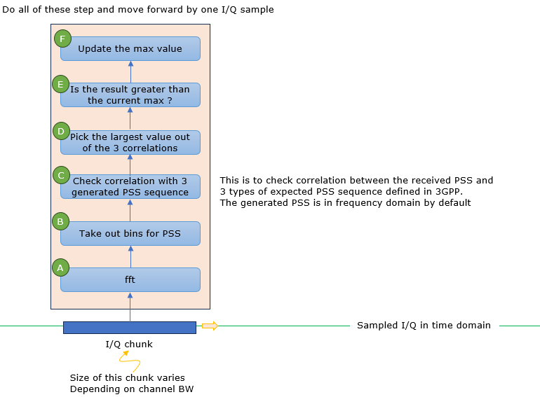
Frequency domain correlation. Steps A to F run for each window, and the window then moves forward by one sample.

Description of what's happening at each step in the illustration goes as follows :

(A) Fast Fourier Transform (FFT) of IQ in a window (chunk): This step converts the time-domain IQ signals in a window, or chunk, into the frequency domain.

(B) Take out bins for PSS: After the FFT, the frequency bins corresponding to the PSS signal are extracted. In LTE, these are the central 62 frequency bins around DC, which contain the PSS signal.

(C) Check Correlation with 3 generated PSS: In this step, the extracted frequency bins are correlated with the three possible PSS sequences that are locally generated and transformed into the frequency domain.

(D) Pick the largest value of the 3 correlations: Once the correlation values are obtained for all three PSS sequences, the maximum correlation value is chosen. This step identifies the specific PSS sequence (out of the three possible ones) that matches the received signal.

(E) Is the result greater than the current max? This step compares the maximum correlation value from step (D) with a predefined threshold or the maximum correlation value from the previous chunk.

(F) Update the max value: If the maximum correlation value from step (D) is larger than the current maximum, this new value is set as the maximum. This updated value then serves as the threshold for the next chunk. If the PSS is successfully detected, it means the 5 ms half-frame boundary is found and frequency synchronization can be established.

The window moves by one sample, so the search is expensive at full rate. At 30.72 MHz, one 5 ms half-frame is 153600 samples. A practical receiver first filters and decimates the signal to 1.92 MHz, enough for the central 72 subcarriers, which cuts the search to 9600 positions.

Time Domain Correlation Method

The time domain method converts the three reference PSS sequences to the time domain once, and then correlates them directly with the received samples. It avoids an FFT for every window, at the cost of preparing the time domain references first.

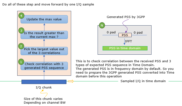
Time domain correlation. Box N prepares each reference PSS with zero padding and an IFFT, and steps 1 to 4 run for each window.

Description of what's happening at each step in the illustration goes as follows :

(1) Check Correlation with 3 generated PSS: In this step, the incoming time-domain IQ samples are correlated with the three possible PSS sequences. These sequences are originally generated in the frequency domain as defined by the LTE standard, then transformed into the time domain for this correlation process. (NOTE : The way in which the PSS is converted to time domain sequence is shown in the box (N))

(2) Pick the largest value of the 3 correlations: Once the correlation values are obtained for all three PSS sequences, the maximum correlation value is chosen. This step identifies the specific PSS sequence (out of the three possible ones) that matches the received signal.

(3) Is the result greater than the current max? This step compares the maximum correlation value from step (2) with a predefined threshold or the maximum correlation value from the previous chunk.

(4) Update the max value: If the maximum correlation value from step (2) is larger than the current maximum, this new value is set as the maximum. This updated value then serves as the threshold for the next chunk. If the PSS is successfully detected, it means the 5 ms half-frame boundary is found and time synchronization can be established.

Box N shows the preparation. The 62 PSS values go on the central subcarriers, the other subcarriers are zeros, and an IFFT gives the time domain sequence. A real receiver usually computes the correlation as an FFT-based convolution, which is what srsran_conv_fft_cc_run_opt() in the list below does.

Source Code in srsUE

You can check out and see how real life implementation of this process in srsUE source code. Followings are the list of functions you would refer to this process (this is based on the code that I downloaded for srs github in Jul 2023)

• \lib\src\phy\sync\pss.c -> int srsran_pss_find_pss()
• \lib\src\phy\utils\convolution.c\srsran_conv_fft_cc_run_opt()
• \lib\src\phy\sync\pss.c -> int srsran_pss_init_fft_offset_decim()
• \lib\src\phy\sync\pss.c -> int srsran_pss_resize()
• \lib\src\phy\sync\pss.c -> int srsran_pss_init_N_id_2()
• \lib\src\phy\sync\pss.c -> int srsran_pss_generate()
• \lib\src\phy\utils\convolution.c\srsran_conv_fft_cc_run_opt()

• PSS gives the 5 ms timing, not the frame start : the SSS resolves subframe 0 from subframe 5.
• Frequency domain method : FFT per window, reference used as defined.
• Time domain method : reference converted once by IFFT, often run as FFT convolution.

Frequency Adjustment with PSS

Once the PSS is found, the UE knows exactly which values it should have received. Any difference between those values and the received ones comes from the channel and from the frequency error of the UE oscillator. So the PSS is also the first reference for frequency correction.

In addition fo finding the timing sync of a subframe / OFDM symbol, the detected PSS provide a very important information.

Frequency Offset Estimation

By comparing the expected PSS (ideal PSS) and the received PSS, we can estimate Frequency Offset. This error can be used to adjust other signals (e.g, SSS) before processing. This offset estimation is crucial in wireless communication for correcting carrier frequency offsets introduced by transmitter-receiver oscillator frequency mismatches or the Doppler effect.

The way to calculate (estimate) the frequency offset can be done by comparing the PSS sequence received and the PSS sequence (i.e, expected sequence) that is generated by the 3GPP algorithm. This comparison and frequency offset can be done in 3 steps as follows.

Step 1 :  Compute the phase difference between each corresponding elements of the received sequence and the expected sequence

Step 2 :  Sum all of the phase difference in step 2. Let's call this as total phase difference

Step 3 :  Convert the total phase difference into frequency offset

This can be explained in more detail with a simple Python script as follows.

Let me look into the code itself.

phase_difference = np.angle(np.dot(received_pss, np.conj(expected_pss)))

This corresponds to Step 1 and Step 2 described above. np.dot(received_pss, np.conj(expected_pss) can be expressed in terms of angular value as follows.

        angle( sum(angle(received_pss) - angle(expected_pss)) )

The minus '-' before angle(expected_pss) is done by taking conj( ) of expected_pss

frequency_offset = (phase_difference / (2 * np.pi)) / time_duration_pss

This line translates the calculated phase difference into the frequency domain to estimate the frequency offset. The factor of 2*πi converts the phase from radians to cycles, 62 is the number of subcarriers used for the PSS in LTE, and sample_rate is the rate at which the PSS signal was sampled.

Phase and frequency are directly related: the change in phase over time is frequency. In the frequency offset estimation function, the phase difference is divided by the time duration of the symbol (which is the number of subcarriers divided by the sample rate), giving us the rate of change of phase, or frequency offset.

In other words, the equation calculates the average change in phase per sample, which is then converted to Hz to represent the frequency offset. This frequency offset represents the difference in frequency between the received PSS and the expected PSS

The function above is a simplified illustration, and two points need care before using it. First, a single correlation phase measures a common phase rotation, not a frequency. The phase-shift example above shows this: a constant rotation of pi/3 changes the angle, but it has no rate. Second, 62 / sample_rate is not the duration of the PSS. The PSS is one OFDM symbol, 2048 samples plus the cyclic prefix at 30.72 MHz, and its useful part lasts about 66.7 microseconds.

A common way to measure frequency from the PSS is to split the time domain correlation into a first half and a second half. The phase difference between the two half-correlations, divided by 2 pi times the time between their centres, gives the frequency offset. With half a symbol, about 33.3 microseconds, between the centres, the estimate is unambiguous up to plus or minus 15 kHz.

• One correlation phase is a phase, not a frequency : it needs a time difference.
• Split-half correlation : phase difference over 33.3 microseconds gives the offset.

Frequency Offset Compensation

Once the frequency offset is calculated (estimated) as explained above, you can use the value to compensate (correct) the frequency offset of other signal (data).

The basic idea is as follows :

Step 1 : Convert the frequency offset to phase shift and generate a rotating factor.

Step 2 : Rotate (compensate) the given signal using the rotating factor

This can be explained by a simple python code as below :

Let me look into the code itself.

time = len(signal) / sample_rate

The time is calculated as the total duration of the signal in seconds. This is done by dividing the number of samples in the signal (len(signal)) by the sample rate (sample_rate).

correction = np.exp(-1j * 2 * np.pi * frequency_offset * time)

The value correction here is the correction factor. This is a complex-valued factor that, when multiplied with the original signal, will correct the frequency offset. The correction factor is computed using the formula for a complex exponential, np.exp(-1j * 2 * np.pi * frequency_offset * time),

• The -1j in the exponential formula represents a negative imaginary unit, and it's used to rotate the signal in the opposite direction of the offset.
• The 2 * np.pi * frequency_offset term inside the exp() represents the angular frequency in radians per second.
• The time is the total duration of the signal in seconds.

corrected_signal = signal * correction

The corrected_signal is then computed by multiplying the original signal with the correction factor. This rotates the signal by the required amount to correct the frequency offset.

NOTE :  The method implemented here is a kind of simplified method. It assumes that all the samples in the data has the same amount of frequency offset. Typically, frequency offset correction involves applying a different correction factor to each sample in the signal (i.e., each sample gets rotated by a different amount), rather than applying the same correction factor to all samples, as is done here. This can be done by computing the correction factor as a function of time for each sample. But this approach is not used in this specific function.

However, if the frequency offset is not constant over the time span of the signal, this method might not fully correct the frequency offset. This is because the method assumes a constant frequency offset over the entire time span of the signal.

In the code, time = len(signal) / sample_rate is one number for the whole signal, so the correction is one constant phase. A frequency offset makes the phase grow linearly with time. The correction for sample m therefore has to be exp(-j 2 pi f m / sample_rate), with m counted from the first sample, which is the per-sample approach the NOTE above describes.

• Correct each sample separately : the phase error grows with time.
• A constant correction : removes a phase offset only.

Reference

[1] Synchronization and Cell Search  

[2] 3GPP TS 36.211 v19.3.0 - clause 6.11.1, Primary synchronization signal, and clause 6.11.2, Secondary synchronization signal