Layer Mapping
This page would deal with the sections highlighed as below (From 3GPP 36.211). Layer Mapping in Rel 8 was relatively simple and intuitive since the number of antenna were only 2 in maximum (the spec itself defined more than 2, but in practice I didn't see any Rel 8 UE or even eNB that support more than 2 antenna). But with
LTE Advanced, especially with Rel 10 and higher, we are seeing more and more UE and Networks supporting more than 2 antenna. Once the number of physical antenna, layer mapping would not look like intuitive and be confusing. So I decided to write a separate page for layer mapping in LTE Advanced. Both tables below are screenshots and neither carries a version stamp, so the last section on this page sets them against 36.211 v19.3.0. One of the two has not moved at all. The other has gained a row.
The drawing below is the whole transmit chain, and the layer mapper is one box in the middle of it. What goes into that box is codewords, and what comes out is layers, which is the only point in the chain where the two names differ.
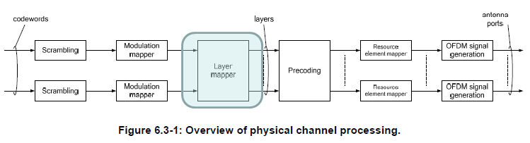
< 36.211 Figure 6.3-1 : Overview of physical channel processing >
Two codewords enter and one layer mapper serves both : scrambling and the modulation mapper each run once per codeword, and the layer mapper is the first box that sees both branches together.
The split after it is by antenna port : precoding feeds a resource element mapper and an OFDM signal generator for each antenna port. The layers the box produced are spread across ports from there on.
The layer count first appears at that box : scrambling and the modulation mapper both work on a codeword, and the number of layers shows up only on the arrows leaving the layer mapper.
The downlink table answers one question: given a number of layers and a number of codewords, which modulation symbol of which codeword goes to which layer. It is long because those two numbers do not move together, and several layer counts can be reached from either one codeword or two.
What follows is the whole of that table, split across three pictures because of its height. The left two columns give the case, the third gives the mapping formula, and the fourth gives the resulting symbol count per layer.

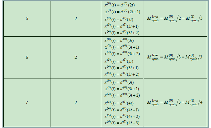
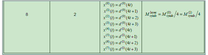
< 36.211 Table 6.3.3.2-1 : Codeword-to-layer mapping for spatial multiplexing >
One codeword can feed more than one layer : the rows for 2, 3 and 4 layers each appear twice, once with one codeword and once with two. 36.211 allows the single codeword case only when there are four cell-specific reference signals, or two or more UE-specific ones.
Past four layers there is always a second codeword : the rows for 5, 6, 7 and 8 layers are all two codeword rows. The shading in the pictures marks them as the ones Release 10 added.
The two codewords need not carry the same number of layers : at 5 layers codeword 0 takes 2 and codeword 1 takes 3, and at 7 layers codeword 0 takes 3 and codeword 1 takes 4. Only the even layer counts divide evenly.
The right hand column is the bookkeeping : it gives the symbol count per layer against the symbol count of each codeword. The 8 layer row reads M(0)symb/4 = M(1)symb/4, so the two codewords have to be equal in length.
An odd layer count forces unequal codewords : the 7 layer row reads M(0)symb/3 = M(1)symb/4, so codeword 1 has to be a third longer than codeword 0 for every layer to hold the same number of symbols.
Just to give you more intuitive understanding of these table shown above, I represented two typical items as illustration.
Following illustration is the case where the number of codeword is 2 and number of layer is 4.

< Two codewords mapped onto four layers >
Each codeword feeds two layers : codeword 0 supplies Layer 0 and Layer 1, and codeword 1 supplies Layer 2 and Layer 3. That is the 4 layer, 2 codeword row of the table drawn out.
The arrows cross because of how the codewords are drawn : each codeword runs right to left in the picture, with d(0)(2i) at the right end. The line to Layer 0 therefore crosses the line to Layer 1.
Following illustration is the case where the number of codeword is 2 and number of layer is 8.
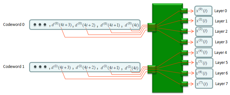
< Two codewords mapped onto eight layers >
Each codeword now feeds four layers : codeword 0 supplies Layers 0 to 3 from d(0)(4i) through d(0)(4i+3), and codeword 1 supplies Layers 4 to 7 the same way.
The index step is the layer count per codeword : four layers per codeword makes the step 4i, where two layers per codeword made it 2i in the drawing above.
Codeword 0 does not reach the upper layers : the two drawings together show that a codeword never spreads across the whole set. It takes a contiguous block, and the second codeword takes the rest.
The uplink keeps the same idea and needs far less of it. Spatial multiplexing on PUSCH arrived in Release 10 and stops at four layers, so the uplink table ends where the downlink one is only half finished. Every row it does carry has a downlink counterpart that reads identically.
The columns below are the same three as the downlink table, and the shading again marks what Release 10 added. Only the top row predates it.
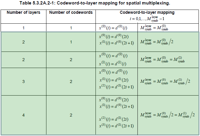
< 36.211 Table 5.3.2A.2-1 : Codeword-to-layer mapping for spatial multiplexing >
The single layer row is the only unshaded one : one codeword on one layer is what the uplink did before Release 10, and every other row in the picture is shaded.
The 3 layer row is the asymmetric one : codeword 0 takes one layer and codeword 1 takes two, so x(0)(i) = d(0)(i) while x(1)(i) = d(1)(2i) and x(2)(i) = d(1)(2i+1).
Only one row here uses a single codeword on several layers : the picture has a 2 layer single codeword row and nothing above it. The downlink table carries 3 layer and 4 layer single codeword rows as well.
That row has a condition on it : 36.211 allows one codeword on more than one layer only when four antenna ports are used for PUSCH.
Neither picture above carries a version stamp, so the first thing worth checking is whether either has moved since. One of them has not changed at all. The other has gained a row, and the reason is a feature that did not exist when the screenshot was taken.
The downlink table is unchanged : 36.211 v19.3.0 Table 6.3.3.2-1 still carries the same eleven rows in the same order, from 1 layer with 1 codeword through to 8 layers with 2 codewords. The three pictures above are current.
The uplink table gained a row : v19.3.0 Table 5.3.2A.2-1 adds 4 layers with 1 codeword, and a note limits it to slot-PUSCH and subslot-PUSCH.
Short TTI is what changed the codeword rule : 36.211 says a single codeword is used for slot-PUSCH and subslot-PUSCH whatever the number of layers. The new row records that exception.
The downlink carries the same exception without a new row : 36.211 adds that for subslot-PDSCH and slot-PDSCH the number of codewords is always one, and the existing single codeword rows already cover it.
Spatial multiplexing is not the only layer mapping : Table 6.3.3.3-1 handles transmit diversity in a table of its own, with one codeword on 2 or 4 layers. Neither picture above shows it.
The conditions on the single codeword rows differ by direction : the downlink needs four cell-specific reference signals or two or more UE-specific ones, and the uplink needs four antenna ports for PUSCH.
One specification carries both tables and the figure. It was resolved at v19.3.0, which is the latest published version at the time of writing.
- 3GPP TS 36.211 v19.3.0, E-UTRA Physical channels and modulation. Clause 6.3.3.2 and Table 6.3.3.2-1 for the downlink, clause 5.3.2A.2 and Table 5.3.2A.2-1 for the uplink, and Figure 6.3-1 for the transmit chain.