In this page, I would do some very basic experiment with a dataset that I created (not a collected data) and try to show you overall procedure on how you design a simple neural network for a given data.
Main purpose of this tutorial is to get familiar with creating a network of different complexity and to see how the number of cells in the in a layer affect the result. As you see in the following list, I will try to classify the same dataset with 4 different neural nets. The main differences among these network is the number of cells in Hidden layer. If you go through all of the experiements, you would get familiar with Matlab syntax constructing a multi-layer network and initializing the network.
- 1 Hidden Layer : 2 Perceptrons in Hidden Layer and 1 Output
- 1 Hidden Layer : 3 Perceptrons in Hidden Layer and 1 Output
- 1 Hidden Layer : 5 Perceptrons in Hidden Layer and 1 Output
- 1 Hidden Layer : 7 Perceptrons in Hidden Layer and 1 Output
1 Hidden Layer : 2 Perceptrons in Hidden Layer, 1 Output
In this example, I will try to classify this data using two layer network : 2 perceptrons in the Hidden layer and one output perceptron. Let's see how well this work.
My intution to this data comparing to previous examples (this and this), the borderline between the two class of dataset looks a little bit complicated and I am not 100% sure if I can categorize this dataset with only 2 neurons in Hidden layer, but let's try anyway. Even if it does not work as I want, I would still learn something about determining network structure and in addtion get more familiar with Matlab Machine Learning Toolbox operation.
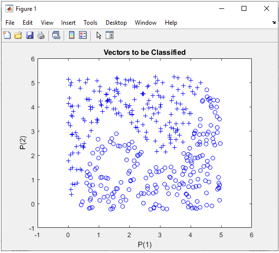
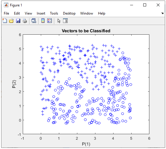
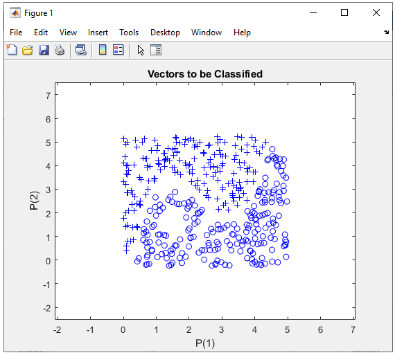
Step 1 : Take a overall distribution of the data plotted as below and try to come up with some idea what kind of neural network you can use. I use the following code to create this dataset. It would not be that difficult to understand the characteristics of dataset from the code itself, but don't spend too much time and effort to understand this part. Just use it as it is.
full_data = [];
xrange = 5;
for i = 1:400
x = xrange * rand(1,1);
y = xrange * rand(1,1);
if y >= 0.6 * (x-1)*(x-2)*(x-4) + 3
y = y + 0.25;
z = 1;
else
y = y - 0.25;
z = 0;
end
full_data = [full_data ; [x y z]];
end
In this case, only two parameters are required to specify a specific data. That's why you can plot the dataset in 2D graph. Of course, in real life situation this would not be a frequent case where you can have this kind of simple dataset, but I would recommend you to try with this type of simple dataset with multiple variations and understand exactly what type of variation you have to make in terms of neural network structure to cope with those variations in data set.
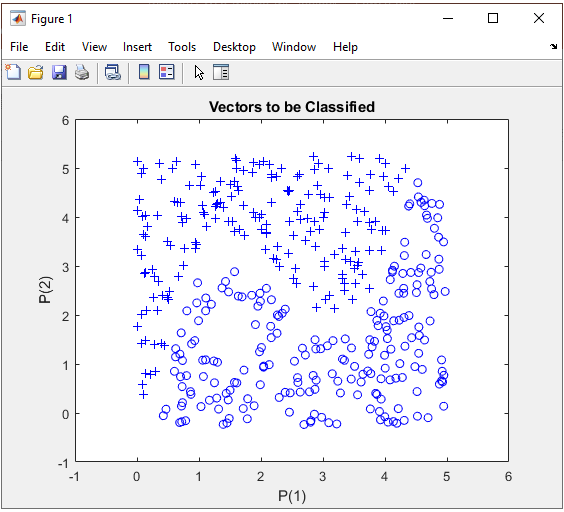
Just taking a quick look at the data, I see there is only two categories of data labeled as '+' and 'o'. So I would need only two input in my neural network.
Then next question is 'would it be possible to classify these two groups of data by a single linear line ?
Obviously Not. It mean that single perceptron and single layer would not solve this classification issue.
Then next question is 'how many output you would need for this classification ? I think I can do this with only one output since there are only two categories.
NOTE : You may use more than one outputs for this classification depending on how you map the output value(s) to each categories of this dataset, but if I can do with one output, what is point of using multiple outputs.
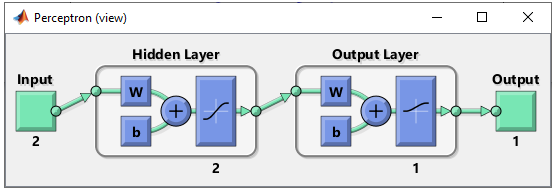
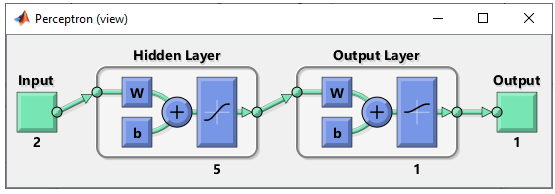
Step 2 : Determine the structure of Neural Nework.
At step 1, I concluded that I would need two inputs and one outputs in the neural network, but the number of layers should be greater than 1. The simplest neural network structure that meets this criteria would be as follows. This network has two inputs and one hidden layer made up of two cells and one output layer made up of one cell. It looks as shown below.
This structure can be created by following code. For further details of meaning of these code, refer to this tutorial.
net = perceptron;
net.numLayers = 2;
net.layers{1}.name = 'Hidden Layer';
net.layers{1}.transferFcn = 'tansig'; % try other transfer function referring here and see how it works.
net.layers{1}.dimensions = 2;
net.layers{2}.name = 'Output Layer';
net.layers{2}.transferFcn = 'logsig'; % try other transfer function referring here and see how it works.
net.layers{2}.dimensions = 1;
Then define the connection between each layers. If you want further details on meaning of these code, refer to this tutorial.
net.layerConnect = [0 0;...
1 0];
net.outputConnect = [0 1];
net.biasConnect = [1;...
1];
net = configure(net,[0; 0],[0]);
Now Initialize the weight and bias of every perceptrons (neurons). If you want further details on meaning of these code, refer to this tutorial.
net.b{1} = [1; ...
1];
net.b{2} = 1;
wi = [1 -0.8; ...
1 -0.8];
net.IW{1,1} = wi;
wo = [1 -0.8];
net.LW{2,1} = wo;
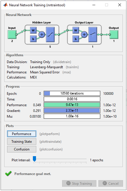
Step 3 : Train the network.
Training a network is done by a single line of code as follows.
[net,tr] = train(net,pList,tList);
Just running this single line of code may nor may not solve your problem. In that case, you may need to tweak the parameters involved in the training process. First tweak the following parameters and try with different activation functions in step 2.
net.trainParam.epochs =2000;
net.trainParam.goal = 10^-7;
net.trainParam.min_grad = 10^-7;
net.trainParam.max_fail = 2;
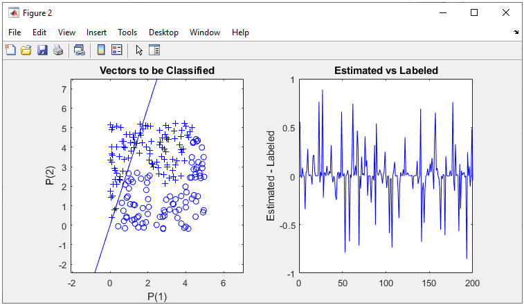
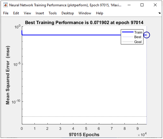
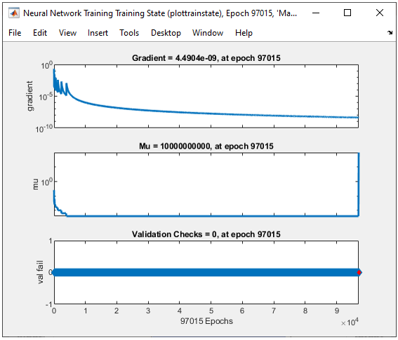
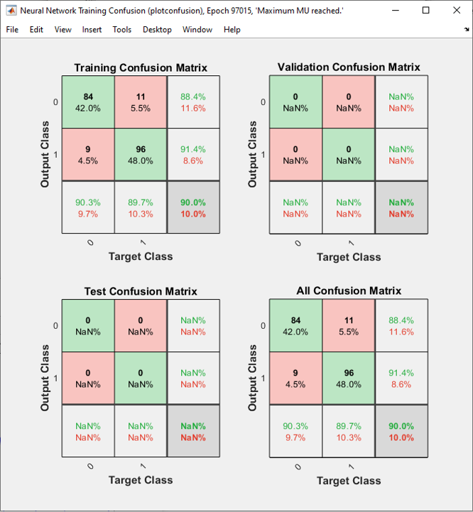
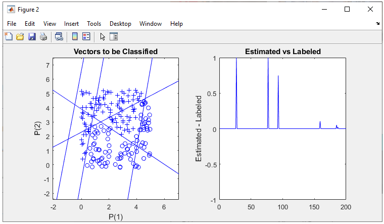
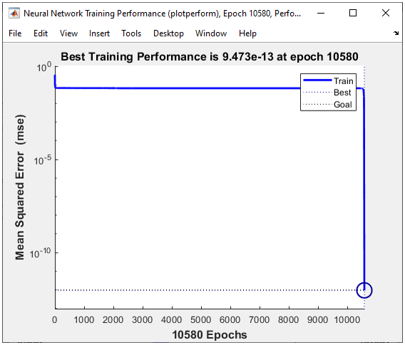
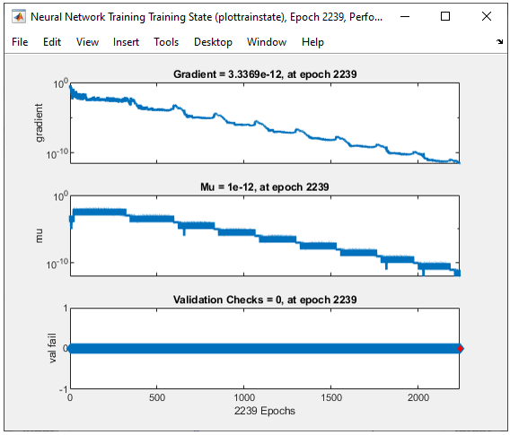
The result in this example is as shown below.
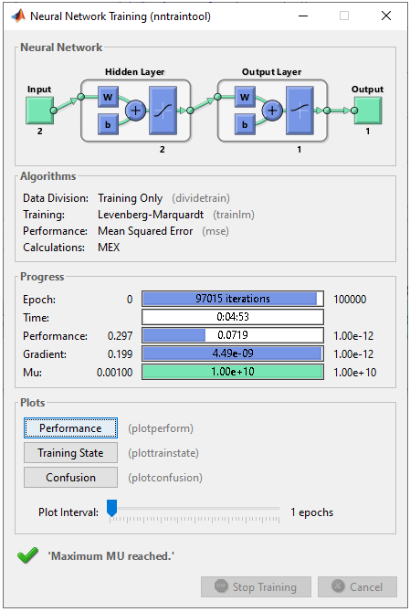
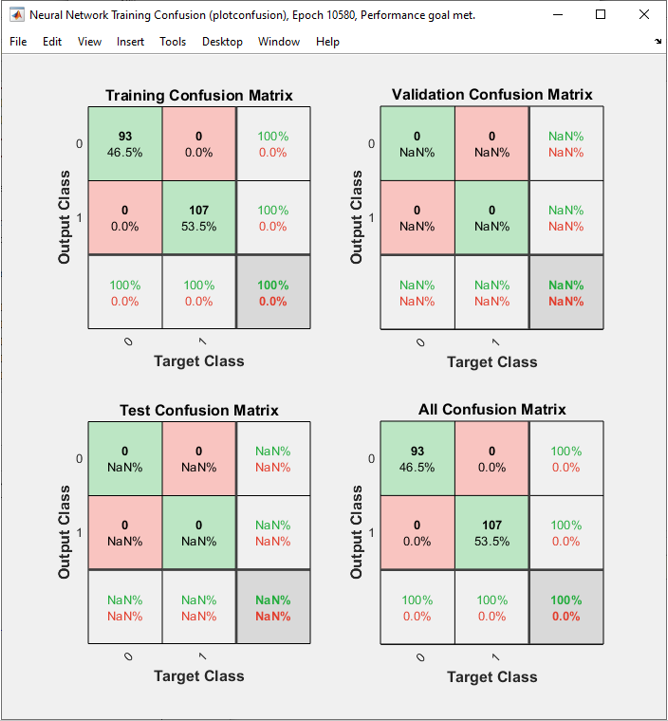
As shown on the left, it seems that the network didn't do good job, and I am happy to find this case which is not working well with this kind of simplet network -:). Good motivation to try with more complicated network.
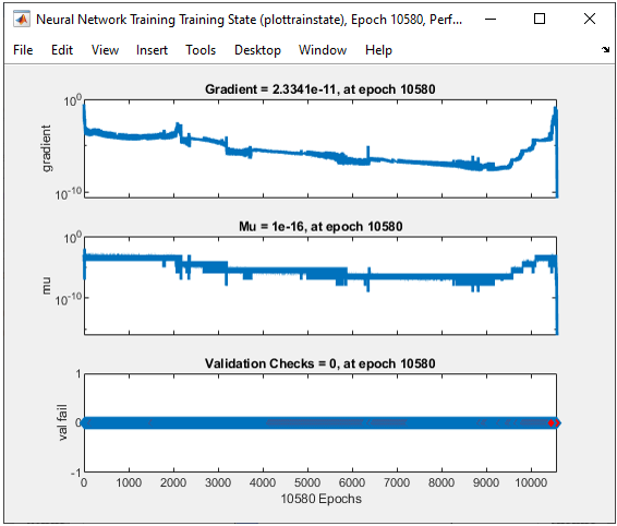
All of the following plots are showing how the training process reaches the target at each iteration. I would not explain on these plots. See if you can understand the performance is not so good from these plots.
|
% Generate Data Set rng(1); full_data = [];
xrange = 5; for i = 1:400
x = xrange * rand(1,1); y = xrange * rand(1,1);
if y >= 0.6 * (x-1)*(x-2)*(x-4) + 3 y = y + 0.25; z = 1; else y = y - 0.25; z = 0; end
full_data = [full_data ; [x y z]];
end
% Split the dataset into Training set and Test Set data_Train = full_data(1:200,:); data_Test = full_data(201:400,:);
figure(1); plotpv([full_data(:,1)'; full_data(:,2)'],full_data(:,3)'); axis([-1 6 -1 6]);
figure(2); set(gcf, 'Position', [100, 100, 750, 350]);
% Initialize Input Vector with Training Dataset pList = [data_Train(:,1)'; data_Train(:,2)']; tList = data_Train(:,3)';
% Build a Neural Net
subplot(1,2,1);
plotpv(pList,tList);
net = perceptron; net.performFcn = 'mse'; net.trainFcn = 'trainlm';
net.numLayers = 2;
net.layers{1}.name = 'Hidden Layer'; net.layers{1}.transferFcn = 'tansig'; net.layers{1}.dimensions = 2;
net.layers{2}.name = 'Output Layer'; net.layers{2}.transferFcn = 'logsig'; net.layers{2}.dimensions = 1;
net.layerConnect = [0 0;... 1 0]; net.outputConnect = [0 1]; net.biasConnect = [1;1];
net = configure(net,[0; 0],[0]);
net.b{1} = [1;... 1]; net.b{2} = 0; wi = [-1.4 -0.8; ... -0.8 -0.1]; net.IW{1,1} = wi; wo = [1 -0.8]; net.LW{2,1} = wo;
% Perform Training
net.trainParam.epochs =100000; net.trainParam.goal = 10^-12; net.trainParam.min_grad = 10^-12; net.trainParam.max_fail = 1; view(net);
[net,tr] = train(net,pList,tList);
% Plot Training Result
for i = 1:length(net.iw{1,1}) plotpc(net.iw{1,1}(i,:),net.b{1}(i,:)); hold on end pList = [data_Test(:,1)'; data_Test(:,2)']; tList = data_Test(:,3)';
subplot(1,2,2);
y = net(pList); plot(y-tList,'b-'); ylim([-1 1]); ylabel('Estimated - Labeled'); title('Estimated vs Labeled'); |
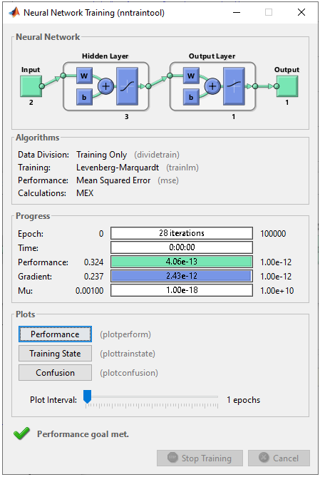
1 Hidden Layer : 3 Perceptrons in Hidden Layer and 1 Output
In this example, I will try to classify this data using two layer network : 3 perceptrons in the Hidden layer and one output perceptron. Let's see how well this work.
The basic logic is exactly same as in previous section. The only difference is that I have one more cell(perceptron) in the hidden layer.
What do you think ? Would it give a better result ?
If it give poorer result, would it be because of this one additional cell in the hidden layer ? or would it be because other training parameters are not optimized properly.
Step 1 : Take a overall distribution of the data plotted as below and try to come up with some idea what kind of neural network you can use. I use the following code to create this dataset. It would not be that difficult to understand the characteristics of dataset from the code itself, but don't spend too much time and effort to understand this part. Just use it as it is.
full_data = [];
xrange = 5;
for i = 1:400
x = xrange * rand(1,1);
y = xrange * rand(1,1);
if y >= 0.6 * (x-1)*(x-2)*(x-4) + 3
y = y + 0.25;
z = 1;
else
y = y - 0.25;
z = 0;
end
full_data = [full_data ; [x y z]];
end
In this case, only two parameters are required to specify a specific data. That's why you can plot the dataset in 2D graph. Of course, in real life situation this would not be a frequent case where you can have this kind of simple dataset, but I would recommend you to try with this type of simple dataset with multiple variations and understand exactly what type of variation you have to make in terms of neural network structure to cope with those variations in data set.
Step 2 : Determine the structure of Neural Nework.
As mentioned above, the purpose of this experiement is to see how the network works when I add one more cell in the hidden layer. So the structure should look as follows.

This structure can be created by following code. For further details of meaning of these code, refer to this tutorial.
net = perceptron;
net.numLayers = 2;
net.layers{1}.name = 'Hidden Layer';
net.layers{1}.transferFcn = 'tansig'; % try other transfer function referring here and see how it works.
net.layers{1}.dimensions = 3;
net.layers{2}.name = 'Output Layer';
net.layers{2}.transferFcn = 'tansig'; % try other transfer function referring here and see how it works.
net.layers{2}.dimensions = 1;
Then define the connection between each layers. If you want further details on meaning of these code, refer to this tutorial.
net.layerConnect = [0 0;...
1 0];
net.outputConnect = [0 1];
net.biasConnect = [1;...
1];
net = configure(net,[0; 0],[0]);
Now Initialize the weight and bias of every perceptrons (neurons). If you want further details on meaning of these code, refer to this tutorial.
net.b{1} = [1; ...
1; ...
1];
net.b{2} = 1;
wi = [1 -0.8; ...
1 -0.8; ...
1 -0.8];
net.IW{1,1} = wi;
wo = [1 -0.8 0.1];
net.LW{2,1} = wo;
Step 3 : Train the network.
Training a network is done by a single line of code as follows.
[net,tr] = train(net,pList,tList);
Just running this single line of code may nor may not solve your problem. In that case, you may need to tweak the parameters involved in the training process. First tweak the following parameters and try with different activation functions in step 2.
net.trainParam.epochs =100000;
net.trainParam.goal = 10^-12;
net.trainParam.min_grad = 10^-12;
net.trainParam.max_fail = 1;
The result in this example is as shown below.
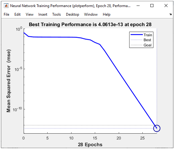
The result is as shown below and you will notice that the network did pretty good job to classify the dataset.
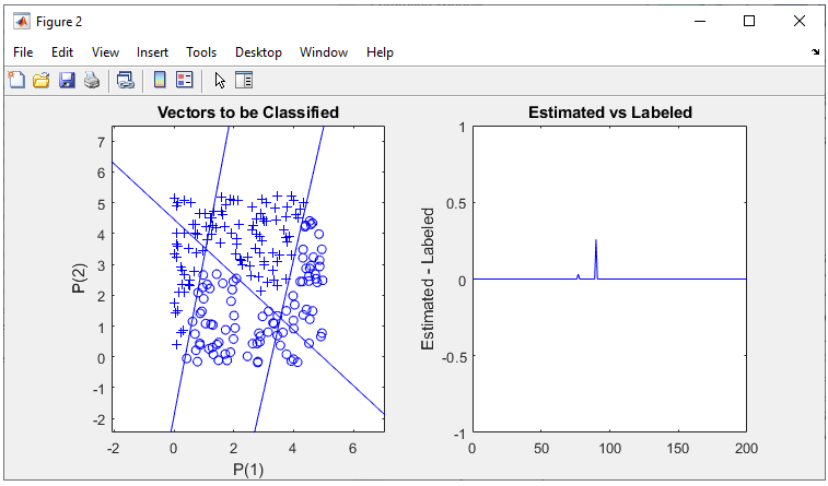
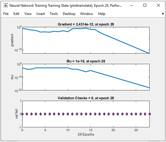
All of the following plots are showing how the training process reaches the target at each iteration. I would not explain on these plots.

|
% Generate Data Set rng(1); full_data = [];
xrange = 5; for i = 1:400
x = xrange * rand(1,1); y = xrange * rand(1,1);
if y >= 0.6 * (x-1)*(x-2)*(x-4) + 3 y = y + 0.25; z = 1; else y = y - 0.25; z = 0; end
full_data = [full_data ; [x y z]];
end
% Split the dataset into Training set and Test Set data_Train = full_data(1:200,:); data_Test = full_data(201:400,:);
% Initialize Input Vector with Training Dataset pList = [data_Train(:,1)'; data_Train(:,2)']; tList = data_Train(:,3)';
figure(1); plotpv([full_data(:,1)'; full_data(:,2)'],full_data(:,3)'); axis([-1 6 -1 6]);
figure(2); set(gcf, 'Position', [100, 100, 750, 350]);
% Build a Neural Net subplot(1,2,1);
plotpv(pList,tList);
net = perceptron; net.performFcn = 'mse'; net.trainFcn = 'trainlm';
net.numLayers = 2;
net.layers{1}.name = 'Hidden Layer'; net.layers{1}.transferFcn = 'tansig'; net.layers{1}.dimensions = 3;
net.layers{2}.name = 'Output Layer'; net.layers{2}.transferFcn = 'logsig'; net.layers{2}.dimensions = 1;
net.layerConnect = [0 0;... 1 0]; net.outputConnect = [0 1]; net.biasConnect = [1;1];
net = configure(net,[0; 0],[0]);
net.b{1} = [1;... 1;... 1]; net.b{2} = 1; wi = [1 -0.8;... 1 -0.8;... 1 -0.8]; net.IW{1,1} = wi; wo = [1 -0.8 0.1]; net.LW{2,1} = wo;
% Perform Training
net.trainParam.epochs =100000; net.trainParam.goal = 10^-12; net.trainParam.min_grad = 10^-12; net.trainParam.max_fail = 1; view(net);
[net,tr] = train(net,pList,tList);
% Plot Training Result for i = 1:length(net.iw{1,1}) plotpc(net.iw{1,1}(i,:),net.b{1}(i,:)); hold on end
% Test the trained Network pList = [data_Test(:,1)'; data_Test(:,2)']; tList = data_Test(:,3)';
subplot(1,2,2);
y = net(pList); plot(y-tList,'b-'); ylim([-1 1]); ylabel('Estimated - Labeled'); title('Estimated vs Labeled'); |
1 Hidden Layer : 5 Perceptrons in Hidden Layer, 1 Output
In this example, I will try to classify this data using two layer network : 5 perceptrons in the Hidden layer and one output perceptron. Let's see how well this work.
The basic logic is exactly same as in previous section. The only difference is that I have more cell(perceptron) in the hidden layer.
What do you think ? Would it give a better result ?
If it give poorer result, would it be because of this one additional cell in the hidden layer ? or would it be because other training parameters are not optimized properly.
Step 1 : Take a overall distribution of the data plotted as below and try to come up with some idea what kind of neural network you can use. I use the following code to create this dataset. It would not be that difficult to understand the characteristics of dataset from the code itself, but don't spend too much time and effort to understand this part. Just use it as it is.
full_data = [];
xrange = 5;
for i = 1:400
x = xrange * rand(1,1);
y = xrange * rand(1,1);
if y >= 0.6 * (x-1)*(x-2)*(x-4) + 3
y = y + 0.25;
z = 1;
else
y = y - 0.25;
z = 0;
end
full_data = [full_data ; [x y z]];
end
In this case, only two parameters are required to specify a specific data. That's why you can plot the dataset in 2D graph. Of course, in real life situation this would not be a frequent case where you can have this kind of simple dataset, but I would recommend you to try with this type of simple dataset with multiple variations and understand exactly what type of variation you have to make in terms of neural network structure to cope with those variations in data set.
Step 2 : Determine the structure of Neural Nework.
As mentioned above, the purpose of this experiement is to see how the network works when I add more cells in the hidden layer. So the structure should look as follows.
This structure can be created by following code. For further details of meaning of these code, refer to this tutorial.
net = perceptron;
net.numLayers = 2;
net.layers{1}.name = 'Hidden Layer';
net.layers{1}.transferFcn = 'tansig'; % try other transfer function referring here and see how it works.
net.layers{1}.dimensions = 5;
net.layers{2}.name = 'Output Layer';
net.layers{2}.transferFcn = 'logsig'; % try other transfer function referring here and see how it works.
net.layers{2}.dimensions = 1;
Then define the connection between each layers. If you want further details on meaning of these code, refer to this tutorial.
net.layerConnect = [0 0;...
1 0];
net.outputConnect = [0 1];
net.biasConnect = [1;...
1];
net = configure(net,[0; 0],[0]);
Now Initialize the weight and bias of every perceptrons (neurons). If you want further details on meaning of these code, refer to this tutorial.
net.b{1} = [1; ...
1; ...
1; ...
1; ...
1];
net.b{2} = 1;
wi = [1 -0.8; ...
1 -0.8; ...
1 -0.8; ...
1 -0.8; ...
1 -0.8];
net.IW{1,1} = wi;
wo = [1 -0.8 0.1 0.1 0.1];
net.LW{2,1} = wo;
Step 3 : Train the network.
Training a network is done by a single line of code as follows.
[net,tr] = train(net,pList,tList);
Just running this single line of code may nor may not solve your problem. In that case, you may need to tweak the parameters involved in the training process. First tweak the following parameters and try with different activation functions in step 2.
net.trainParam.epochs =100000;
net.trainParam.goal = 10^-12;
net.trainParam.min_grad = 10^-12;
net.trainParam.max_fail = 1;
The result in this example is as shown below.
As shown belw, the performance is not bad but a little bit worse then previous one (i.e, 3 neurons in Hidden layer). Why ? Would this be because I used too many neurons that led to overfitting ? or because parameters are not properly optimized ?
All of the following plots are showing how the training process reaches the target at each iteration. I would not explain on these plots.
|
% Generate Data Set rng(1); full_data = [];
xrange = 5; for i = 1:400
x = xrange * rand(1,1); y = xrange * rand(1,1);
if y >= 0.6 * (x-1)*(x-2)*(x-4) + 3 y = y + 0.25; z = 1; else y = y - 0.25; z = 0; end
full_data = [full_data ; [x y z]];
end
% Split the dataset into Training set and Test Set data_Train = full_data(1:200,:); data_Test = full_data(201:400,:);
figure(1); plotpv([full_data(:,1)'; full_data(:,2)'],full_data(:,3)'); axis([-1 6 -1 6]);
figure(2); set(gcf, 'Position', [100, 100, 750, 350]);
% Initialize Input Vector with Training Dataset pList = [data_Train(:,1)'; data_Train(:,2)']; tList = data_Train(:,3)';
% Build a Neural Net subplot(1,2,1);
plotpv(pList,tList);
net = perceptron; net.performFcn = 'mse'; net.trainFcn = 'trainlm';
net.numLayers = 2;
net.layers{1}.name = 'Hidden Layer'; net.layers{1}.transferFcn = 'tansig'; net.layers{1}.dimensions = 5;
net.layers{2}.name = 'Output Layer'; net.layers{2}.transferFcn = 'logsig'; net.layers{2}.dimensions = 1;
net.layerConnect = [0 0;... 1 0]; net.outputConnect = [0 1]; net.biasConnect = [1;1];
net = configure(net,[0; 0],[0]);
net.b{1} = [1; ... 1; ... 1; ... 1; ... 1]; net.b{2} = 1; wi = [1 -0.8;... 1 -0.8;... 1 -0.8;... 1 -0.8;... 1 -0.8]; net.IW{1,1} = wi; wo = [1 -0.8 0.1 0.1 0.1]; net.LW{2,1} = wo;
% Perform Training
net.trainParam.epochs =100000; net.trainParam.goal = 10^-12; net.trainParam.min_grad = 10^-12; net.trainParam.max_fail = 1; %net.trainParam.mu = 5; %net.trainParam.mu_dec = 1.0; %net.trainParam.mu_inc = 3.0;
view(net);
[net,tr] = train(net,pList,tList);
% Plot Training Result for i = 1:length(net.iw{1,1}) plotpc(net.iw{1,1}(i,:),net.b{1}(i,:)); hold on end
pList = [data_Test(:,1)'; data_Test(:,2)']; tList = data_Test(:,3)';
subplot(1,2,2);
y = net(pList); plot(y-tList,'b-'); ylim([-1 1]); ylabel('Estimated - Labeled'); title('Estimated vs Labeled'); |
1 Hidden Layer : 7 Perceptrons in Hiddel Layer, 1 Output
In this example, I will try to classify this data using two layer network : 7 perceptrons in the Hidden layer and one output perceptron. Let's see how well this work.
The basic logic is exactly same as in previous section. The only difference is that I have more cell(perceptron) in the hidden layer.
What do you think ? Would it give a better result ?
If it give poorer result, would it be because of this one additional cell in the hidden layer ? or would it be because other training parameters are not optimized properly.
Step 1 : Take a overall distribution of the data plotted as below and try to come up with some idea what kind of neural network you can use. I use the following code to create this dataset. It would not be that difficult to understand the characteristics of dataset from the code itself, but don't spend too much time and effort to understand this part. Just use it as it is.
full_data = [];
xrange = 5;
for i = 1:400
x = xrange * rand(1,1);
y = xrange * rand(1,1);
if y >= 0.6 * (x-1)*(x-2)*(x-4) + 3
y = y + 0.25;
z = 1;
else
y = y - 0.25;
z = 0;
end
full_data = [full_data ; [x y z]];
end
In this case, only two parameters are required to specify a specific data. That's why you can plot the dataset in 2D graph. Of course, in real life situation this would not be a frequent case where you can have this kind of simple dataset, but I would recommend you to try with this type of simple dataset with multiple variations and understand exactly what type of variation you have to make in terms of neural network structure to cope with those variations in data set.
Step 2 : Determine the structure of Neural Nework.
As mentioned above, the purpose of this experiement is to see how the network works when I add more cells in the hidden layer. So the structure should look as follows.
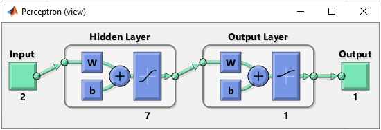
This structure can be created by following code. For further details of meaning of these code, refer to this tutorial.
net = perceptron;
net.numLayers = 2;
net.layers{1}.name = 'Hidden Layer';
net.layers{1}.transferFcn = 'tansig'; % try other transfer function referring here and see how it works.
net.layers{1}.dimensions = 7;
net.layers{2}.name = 'Output Layer';
net.layers{2}.transferFcn = 'logsig'; % try other transfer function referring here and see how it works.
net.layers{2}.dimensions = 1;
Then define the connection between each layers. If you want further details on meaning of these code, refer to this tutorial.
net.layerConnect = [0 0;...
1 0];
net.outputConnect = [0 1];
net.biasConnect = [1;...
1];
net = configure(net,[0; 0],[0]);
Now Initialize the weight and bias of every perceptrons (neurons). If you want further details on meaning of these code, refer to this tutorial.
net.b{1} = [1; ...
1; ...
1; ...
1; ...
1; ...
1; ...
1];
net.b{2} = 1;
wi = [1 -0.8; ...
1 -0.8; ...
1 -0.8; ...
1 -0.8; ...
1 -0.8; ...
1 -0.8; ...
1 -0.8];
net.IW{1,1} = wi;
wo = [1 -0.8 0.1 0.1 0.1 0.1 0.1];
net.LW{2,1} = wo;
Step 3 : Train the network.
Training a network is done by a single line of code as follows.
[net,tr] = train(net,pList,tList);
Just running this single line of code may nor may not solve your problem. In that case, you may need to tweak the parameters involved in the training process. First tweak the following parameters and try with different activation functions in step 2.
net.trainParam.epochs =100000;
net.trainParam.goal = 10^-12;
net.trainParam.min_grad = 10^-12;
net.trainParam.max_fail = 1;
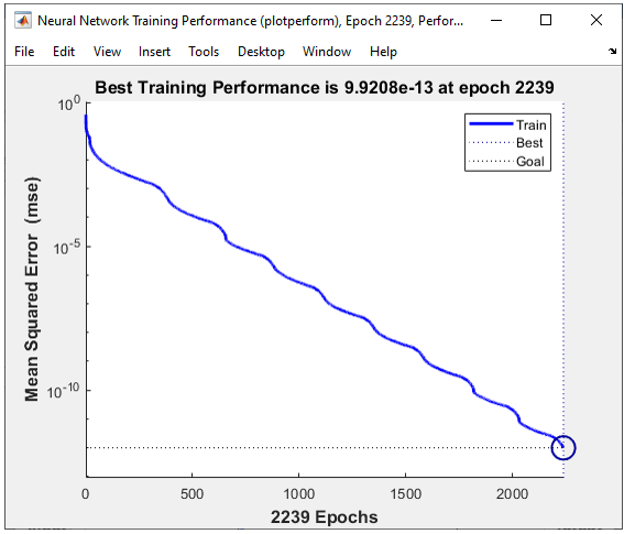
The result in this example is as shown below.
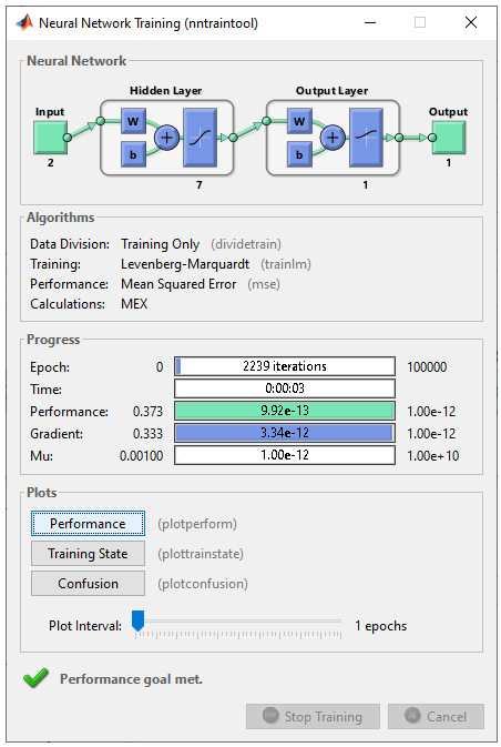
As shown below, the performance is better than previous one (5 neuron in Hidden layer) and similar result as 3 neuron in Hidden layer case.
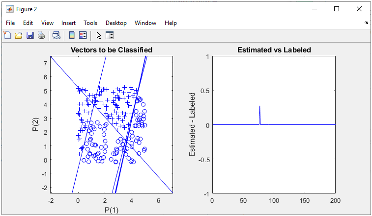
All of the following plots are showing how the training process reaches the target at each iteration. I would not explain on these plots.

|
% Generate Data Set rng(1); full_data = [];
xrange = 5; for i = 1:400
x = xrange * rand(1,1); y = xrange * rand(1,1);
if y >= 0.6 * (x-1)*(x-2)*(x-4) + 3 y = y + 0.25; z = 1; else y = y - 0.25; z = 0; end
full_data = [full_data ; [x y z]];
end
% Split the dataset into Training set and Test Set data_Train = full_data(1:200,:); data_Test = full_data(201:400,:);
% Initialize Input Vector with Training Dataset pList = [data_Train(:,1)'; data_Train(:,2)']; tList = data_Train(:,3)';
figure(1); plotpv([full_data(:,1)'; full_data(:,2)'],full_data(:,3)');
figure(2); set(gcf, 'Position', [100, 100, 750, 350]);
% Build a Neural Net subplot(1,2,1);
plotpv(pList,tList);
net = perceptron; net.performFcn = 'mse'; net.trainFcn = 'trainlm';
net.numLayers = 2;
net.layers{1}.name = 'Hidden Layer'; net.layers{1}.transferFcn = 'tansig'; net.layers{1}.dimensions = 7;
net.layers{2}.name = 'Output Layer'; net.layers{2}.transferFcn = 'logsig'; net.layers{2}.dimensions = 1;
net.layerConnect = [0 0;... 1 0]; net.outputConnect = [0 1]; net.biasConnect = [1;1];
net = configure(net,[0; 0],[0]);
net.b{1} = [1;... 1;... 1;... 1;... 1;... 1;... 1]; net.b{2} = 1; wi = [1 -0.8;... 1 -0.8;... 1 -0.8;... 1 -0.8;... 1 -0.8;... 1 -0.8;... 1 -0.8]; net.IW{1,1} = wi; wo = [1 -0.8 0.1 0.1 0.1 0.1 0.1]; net.LW{2,1} = wo;
% Perform Training
net.trainParam.epochs =100000; net.trainParam.goal = 10^-12; net.trainParam.min_grad = 10^-12; net.trainParam.max_fail = 1; %net.trainParam.mu = 5; %net.trainParam.mu_dec = 1.0; %net.trainParam.mu_inc = 3.0;
view(net);
[net,tr] = train(net,pList,tList);
% Plot Training Result for i = 1:length(net.iw{1,1}) plotpc(net.iw{1,1}(i,:),net.b{1}(i,:)); hold on end
pList = [data_Test(:,1)'; data_Test(:,2)']; tList = data_Test(:,3)';
subplot(1,2,2);
y = net(pList); plot(y-tList,'b-'); ylim([-1 1]); ylabel('Estimated - Labeled'); title('Estimated vs Labeled'); |
Next Step :