Machine Learning  

2D Convolution 

Convolution is a special operation that has mostly been used in control theory and digital signal processing. In these application, the convolution is performed with 1 dimensional data (e.g, time serious data) as explained and shown in my convolution page and various animated examples in my visual note www.slide4math.com. And later the concept of convolution was extended to 2D and has been very widely used for various image processing (e.g, edge detection, noise filtering etc). In this page, I will explain on how the 2D convolution works.

Before you go through the explanation of calculation process, check this page and run animation.. and see if it make sense to you. If you have even a very basic understanding on the concept of 2D convolution, you would have pretty clear understanding on 2D convolution from the animation. If you have difficulties in making a clear sense out of the animation, read through following explanation and then run the animation again.

The 2D convolution goes as follows.

Step 1 : Chose a specific size of filter (also called a kernel) with the specific value. In this example, I will use a kernel with the size of 3x3.

NOTE : In image processing, usually we put a specific values into the filter depending on the purpose of the processing (like edge detection or noise filtering). In case of neural network (CNN), we usually initialize the filter with random values and the element values of the filter gets updated with different values as part of learning process (back propagation).

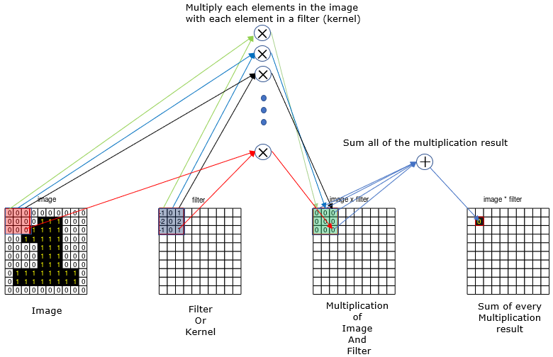
Step 2 : Align the filter to the top left corner of the image as shown below. and do the folliwing operations.

i) multiply each element of the filter with the values at the corresponding locations in the image. (In this example, you need to do 9 multiplication since the size of the filter is 9 (3x3).

ii) sum all of he multiplication example (In this example, sum the 9 values).

iii) write down the summation result onto the corresponding location (the center of the filter) on the result array.

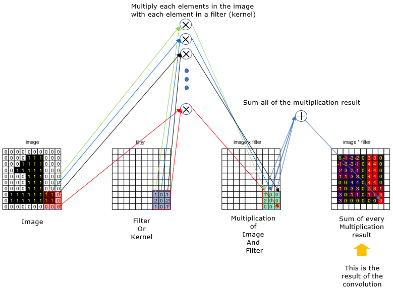
Step 3 : Shift the kernel by one step to the right and do the same thing as shown below.

NOTE : In case of image processing, we shift kernel by single element almost always, but in machine learning application we may shift more than one element (like 2, 3 or more). This shifting interval is called stride.

Step 4 : Repeat the step 3 until the kernel reach to the right end of the image and then shift to the left end and step one element down in vertical direction. this animation will show you clearly on how this kernel shifting goes. Keep doing this process until the kernel reaches right bottom corner of the image as shown below.

Reference :