|
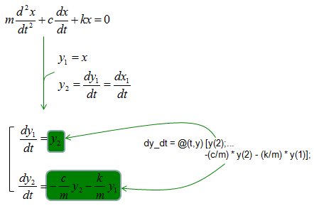
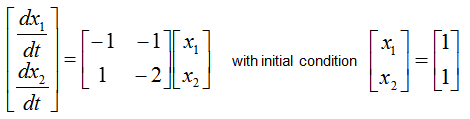
Differential Equation
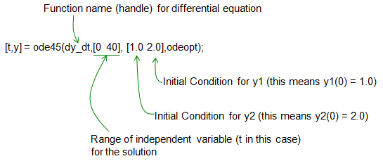
ODE45
Lsim-State Space Model
Step
ode45 - 1st order
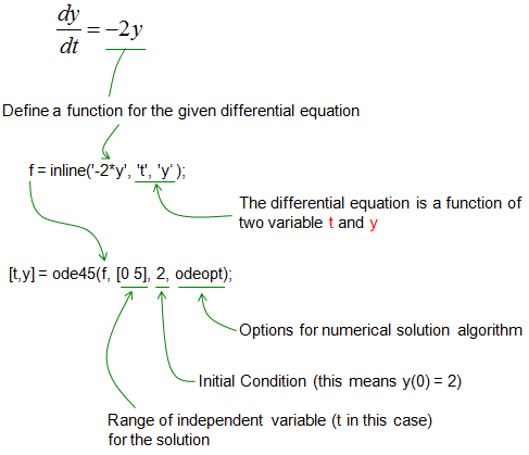
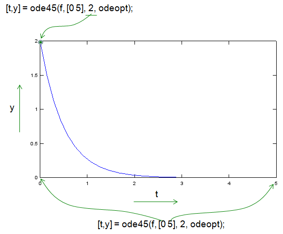
Ex)
|
Input
|
f = inline('-2*y','t','y');
odeopt = odeset ('RelTol', 0.00001, 'AbsTol', 0.00001,'InitialStep',0.5,'MaxStep',0.5);
[t,y] = ode45(f,[0 5],2,odeopt);
plot(t,y)
|
|
Output
|
|
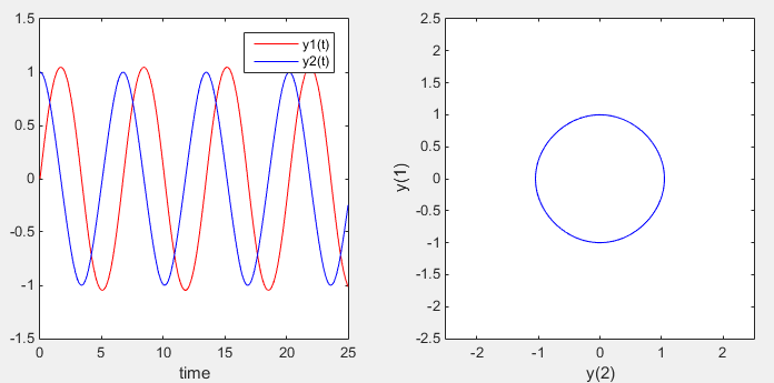
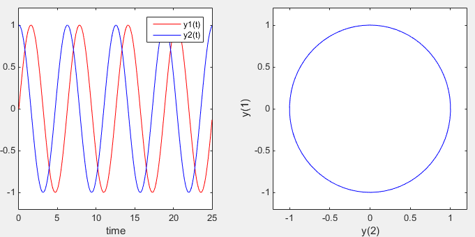
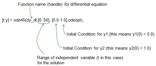
ode45 - Undamped Pendulum
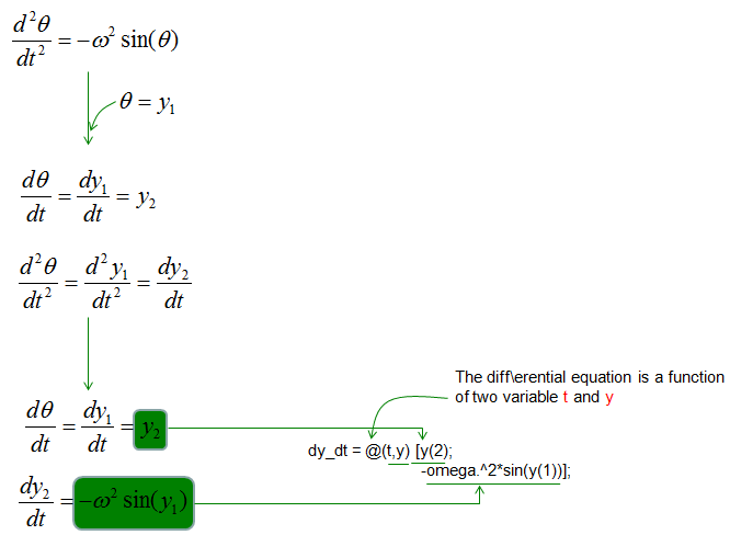
Ex 1)
|
Input
|
%Save the following contents in a .m file and run the .m file
omega = 1;
dy_dt = @(t,y) [y(2);...
-omega.^2*sin(y(1))];
odeopt = odeset ('RelTol', 0.00001, 'AbsTol', 0.00001,'InitialStep',0.5,'MaxStep',0.5);
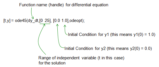
[t,y] = ode45(dy_dt,[0 25], [0.0 1.0],odeopt);
subplot(1,2,1);plot(t,y(:,1),'r-',t,y(:,2),'b-');xlabel('time'); legend('y1(t)','y2(t)');
subplot(1,2,2);plot(y(:,1),y(:,2),'b-'); axis([-2.5 2.5 -2.5 2.5]); xlabel('y(2)');ylabel('y(1)');
|
|
Output
|
|
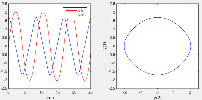
Ex 2) If you change the initial condition, you would get different result (a little bit distorted circle)
|
Input
|
%Save the following contents in a .m file and run the .m file
omega = 1;
dy_dt = @(t,y) [y(2);...
-omega.^2*sin(y(1))];
odeopt = odeset ('RelTol', 0.00001, 'AbsTol', 0.00001,'InitialStep',0.5,'MaxStep',0.5);
[t,y] = ode45(dy_dt,[0 25], [0.0 1.7],odeopt);
subplot(1,2,1);plot(t,y(:,1),'r-',t,y(:,2),'b-'); xlabel('time'); legend('y1(t)','y2(t)');
subplot(1,2,2);plot(y(:,1),y(:,2),'b-'); xlabel('y(2)');ylabel('y(1)');axis([-2.5 2.5 -2.5 2.5]);
|
|
Output
|
|
ode45 - Single Spring Mass- Undamped
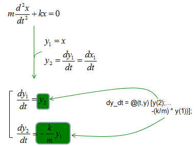
Ex)
|
Input
|
%Save the following contents in a .m file and run the .m file
m = 1;
k = 1;
dy_dt = @(t,y) [y(2);...
-(k/m) * y(1) ];
odeopt = odeset ('RelTol', 0.00001, 'AbsTol', 0.00001,'InitialStep',0.5,'MaxStep',0.5);
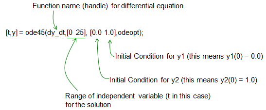
[t,y] = ode45(dy_dt,[0 25], [0.0 1.0],odeopt);
subplot(1,2,1);plot(t,y(:,1),'r-',t,y(:,2),'b-'); xlabel('time'); ylim([-1.2 1.2]); legend('y1(t)','y2(t)');
subplot(1,2,2);plot(y(:,1),y(:,2),'b-'); xlabel('y(2)');ylabel('y(1)'); xlim([-1.2 1.2]); ylim([-1.2 1.2]);
|
|
Output
|
|
ode45 - Single Spring Mass- Damped
Ex)
|
Input
|
%Save the following contents in a .m file and run the .m file
m = 1;
k = 1;
c = 0.3;
dy_dt = @(t,y) [y(2);...
-(c/m) * y(2) - (k/m) * y(1) ];
odeopt = odeset ('RelTol', 0.00001, 'AbsTol', 0.00001,'InitialStep',0.5,'MaxStep',0.5);
[t,y] = ode45(dy_dt,[0 25], [0.0 1.0],odeopt);
subplot(1,2,1);plot(t,y(:,1),'r-',t,y(:,2),'b-'); xlabel('time'); ylim([-1.2 1.2]); legend('y1(t)','y2(t)');
subplot(1,2,2);plot(y(:,1),y(:,2),'b-'); xlabel('y(2)');ylabel('y(1)'); xlim([-1.2 1.2]); ylim([-1.2 1.2]);
|
|
Output
|
|
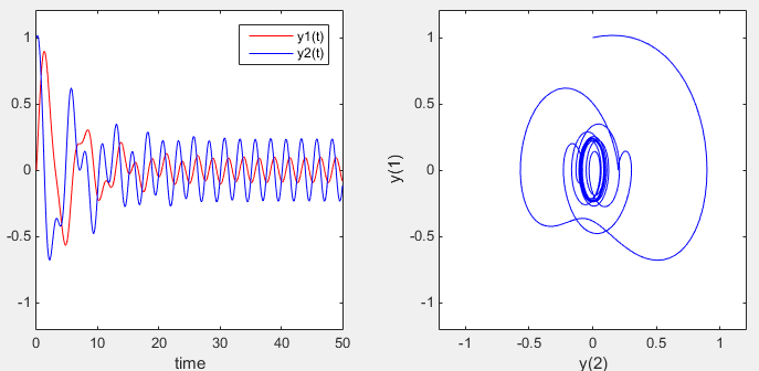
ode45 - Single Spring Mass- Damped and External Force
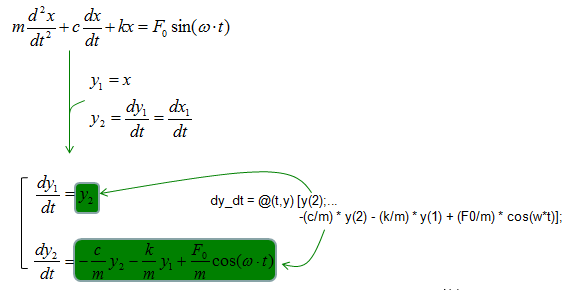
Ex)
|
Input
|
%Save the following contents in a .m file and run the .m file
m = 1;
k = 1;
c = 0.3;
F0 = 0.5;
w = 2.5;
dy_dt = @(t,y) [y(2);...
-(c/m) * y(2) - (k/m) * y(1) + (F0/m) * cos(w*t)];
odeopt = odeset ('RelTol', 0.00001, 'AbsTol', 0.00001,'InitialStep',0.5,'MaxStep',0.5);
[t,y] = ode45(dy_dt,[0 50], [0.0 1.0],odeopt);
subplot(1,2,1);plot(t,y(:,1),'r-',t,y(:,2),'b-'); xlabel('time'); ylim([-1.2 1.2]); legend('y1(t)','y2(t)');
subplot(1,2,2);plot(y(:,1),y(:,2),'b-'); xlabel('y(2)');ylabel('y(1)'); xlim([-1.2 1.2]); ylim([-1.2 1.2]);
|
|
Output
|
|
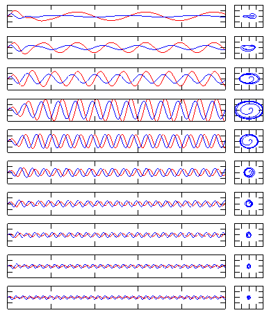
ode45 - Single Spring Mass- Damped and External Force with Frequency Sweep
Ex)
|
Input
|
%Save the following contents in a .m file and run the .m file
m = 1.0;
k = 0.7;
c = 0.3;
F0 = 0.5;
tmax = 100;
yinit = 0.0;
for i = 1:10
w = 0.2 * i;
dy_dt = @(t,y) [y(2);...
-(c/m) * y(2) - (k/m) * y(1) + (F0/m) * cos(w*t)];
odeopt = odeset ('RelTol', 0.00001, 'AbsTol', 0.00001,'InitialStep',0.5,'MaxStep',0.5);
[t,y] = ode45(dy_dt,[0 tmax], [0.0 yinit],odeopt);
subplot(10,7,[(i*7-6) (i*7-1)] );plot(t,y(:,1),'r-',t,y(:,2),'b-');
ylim([-2 2]); set(gca,'xticklabel',[]);set(gca,'yticklabel',[]);
subplot(10,7,i*7);plot(y(:,1),y(:,2),'b-');
xlim([-2 2]); ylim([-2 2]); set(gca,'xticklabel',[]);set(gca,'yticklabel',[]);
end;
|
|
Output
|
|
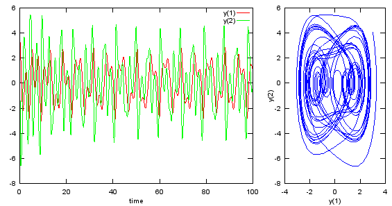
ode45 - 1s Order System Equation- Lorenz Attractor
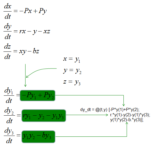
Ex)
|
Input
|
%Save the following contents in a .m file and run the .m file
P = 10;
r = 28;
b = 8/3;
dy_dt = @(t,y) [-P*y(1)+P*y(2);...
r.*y(1)-y(2)-y(1)*y(3);...
y(1)*y(2)-b.*y(3)];
odeopt = odeset ('RelTol', 0.00001, 'AbsTol', 0.00001,'InitialStep',0.5,'MaxStep',0.5);
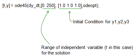
[t,y] = ode45(dy_dt,[0 250], [1.0 1.0 1.0],odeopt);
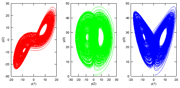
subplot(1,3,1);plot(y(:,1),y(:,2),'r-'); xlabel('y(1)'); ylabel('y(2)');
subplot(1,3,2);plot(y(:,2),y(:,3),'g-'); xlabel('y(2)'); ylabel('y(3)');
subplot(1,3,3);plot(y(:,1),y(:,3),'b-'); xlabel('y(1)'); ylabel('y(3)');
|
|
Output
|
|
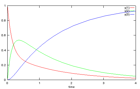
ode45 - Chemical Reaction
Ex)
|
Input
|
%Save the following contents in a .m file and run the .m file
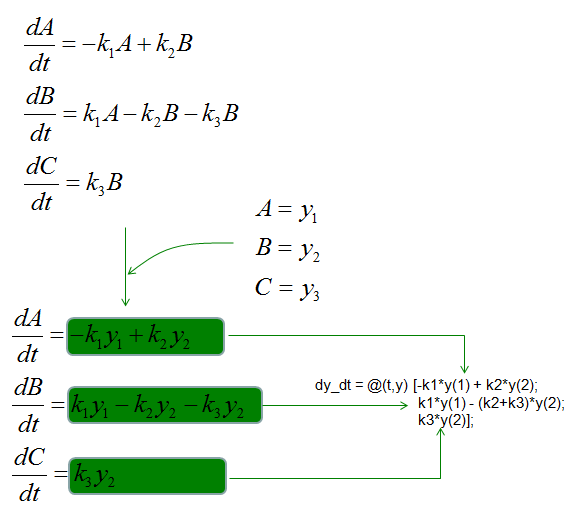
k1 = 5;
k2 = 2;
k3 = 1;
dy_dt = @(t,y) [-k1*y(1) + k2*y(2);
k1*y(1) - (k2+k3)*y(2);
k3*y(2)];
odeopt = odeset ('RelTol', 0.00001, 'AbsTol', 0.00001,'InitialStep',0.5,'MaxStep',0.5);
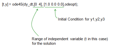
[t,y] = ode45(dy_dt,[0 4], [1.0 0.0 0.0],odeopt);
plot(t,y(:,1),'r-',t,y(:,2),'g-',t,y(:,3),'b-'); xlabel('time'); legend('y(1)','y(2)','y(3)');
|
|
Output
|
|
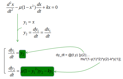
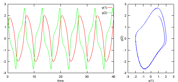
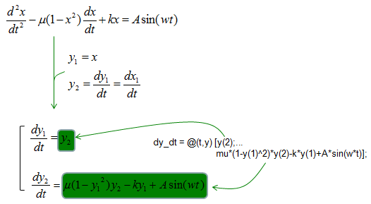
Ode45 - Vander Pol Oscillator
Ex)
|
Input
|
%Save the following contents in a .m file and run the .m file
mu = 1;
k = 1;
dy_dt = @(t,y) [y(2);...
mu*(1-y(1)^2)*y(2)-k*y(1)];
odeopt = odeset ('RelTol', 0.00001, 'AbsTol', 0.00001,'InitialStep',0.5,'MaxStep',0.5);
[t,y] = ode45(dy_dt,[0 40], [1.0 2.0],odeopt);
subplot(1,3,[1 2]);plot(t,y(:,1),'r-',t,y(:,2),'g-'); xlabel('time'); legend('y(1)','y(2)');
subplot(1,3,3);plot(y(:,1),y(:,2)); xlabel('y(1)'); ylabel('y(2)');
|
|
Output
|
|
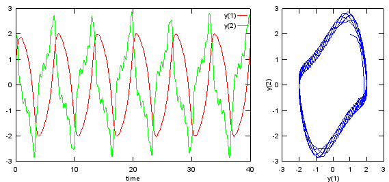
Ode45 - Vander Pol Oscillator with External Force
Ex)
|
Input
|
%Save the following contents in a .m file and run the .m file
mu = 1;
k = 1;
A = 2.0;
w = 10;
dy_dt = @(t,y) [y(2);...
mu*(1-y(1)^2)*y(2)-k*y(1) + A*sin(w*t)];
odeopt = odeset ('RelTol', 0.00001, 'AbsTol', 0.00001,'InitialStep',0.5,'MaxStep',0.5);
[t,y] = ode45(dy_dt,[0 40], [1.0 2.0],odeopt);
subplot(1,3,[1 2]);plot(t,y(:,1),'r-',t,y(:,2),'g-'); xlabel('time'); legend('y(1)','y(2)');
subplot(1,3,3);plot(y(:,1),y(:,2)); xlabel('y(1)'); ylabel('y(2)');
|
|
Output
|
|
Ode45 - Duffing Oscillator
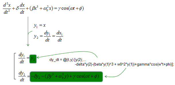
Ex)
|
Input
|
%Save the following contents in a .m file and run the .m file
delta = 0.06;
beta = 1.0;
w0 = 1.0;
w = 1.0;
gamma = 6.0;
phi = 0;
dy_dt = @(t,y) [y(2);...
-delta*y(2)-(beta*y(1)^3 + w0^2*y(1))+gamma*cos(w*t+phi)];
odeopt = odeset ('RelTol', 0.00001, 'AbsTol', 0.00001,'InitialStep',0.5,'MaxStep',0.5);
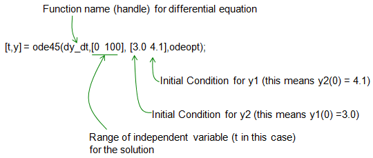
[t,y] = ode45(dy_dt,[0 100], [3.0 4.1],odeopt);
subplot(1,3,[1 2]);plot(t,y(:,1),'r-',t,y(:,2),'g-'); xlabel('time'); legend('y(1)','y(2)');
subplot(1,3,3);plot(y(:,1),y(:,2)); xlabel('y(1)'); ylabel('y(2)');
|
|
Output
|
|
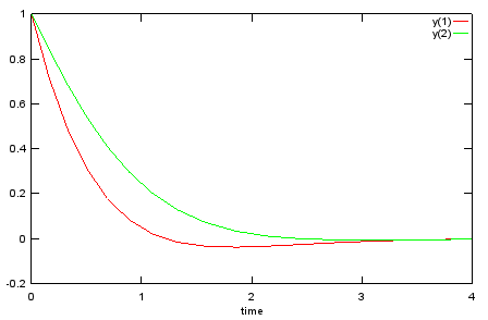
Ode45 - Matrix Equation - 2 x 2
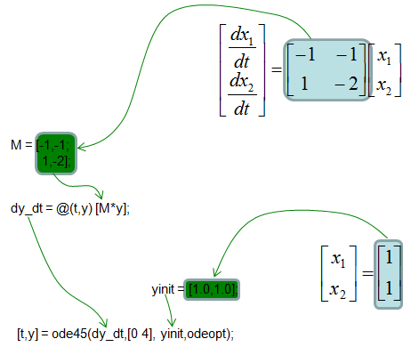
Ex)
|
Input
|
%Save the following contents in a .m file and run the .m file
M = [-1,-1;...
1,-2];
yinit = [1.0,1.0];
dy_dt = @(t,y) [M*y];
odeopt = odeset ('RelTol', 0.00001, 'AbsTol', 0.00001,'InitialStep',0.5,'MaxStep',0.5);
[t,y] = ode45(dy_dt,[0 4], yinit,odeopt);
plot(t,y(:,1),'r-',t,y(:,2),'g-'); xlabel('time'); legend('y(1)','y(2)');
|
|
Output
|
|
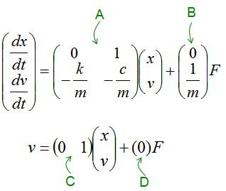
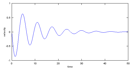
Lsim - Damped Spring
Ex) See Damped Spring Example in Differential Equation page for the description of the model.
|
Input
|
% This is tested on Octave. It would not work on Matlab (tested on Matlab 2014).
m = 1;
c = 0.2;
k = 1;
A = [0 1;-k/m -c/m];
B = [0 ; 1/m];
C = [0 1];
D = [0];
t = 0:0.1:50;
u = zeros(length(t),1);
x0 = [1 0];
sys = ss(A,B,C,0);
[y,t,x] = lsim(sys,u,t,x0);
plot(t,y);xlabel('time');ylabel('velocity');
|
|
Output
|
|
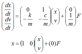
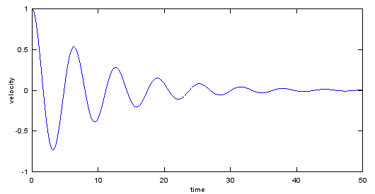
Ex)
|
Input
|
% This is tested on Octave. It would not work on Matlab (tested on Matlab 2014).
m = 1;
c = 0.2;
k = 1;
A = [0 1;-k/m -c/m];
B = [0 ; 1/m];
C = [1 0];
D = [0];
t = 0:0.1:50;
u = zeros(length(t),1);
x0 = [1 0];
sys = ss(A,B,C,0);
[y,t,x] = lsim(sys,u,t,x0);
plot(t,y);xlabel('time');ylabel('velocity');
|
|
Output
|
|
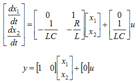
Lsim - RLC Circuit
Ex) See RLC Circuit Example in Differential Equation page for the description of the model.
|
Input
|
% This is tested on Octave. It would not work on Matlab (tested on Matlab 2014).
R = 1;
L = 0.1;
C = 0.01;
A = [0 1;-1/(L*C) -R/L];
B = [0 ; 1/(L*C)];
C = [1 0];
D = [0];
t = 0:0.01:10;
u = ones(length(t),1);
u(200:400) = 0;
x0 = [1 0];
sys = ss(A,B,C,D);
[y,t,x] = lsim(sys,u,t,x0);
plot(t,y,'r-',t,u,'b--');xlabel('time');ylabel('voltage');legend('v2(t)','u(t)');
|
|
Output
|
|
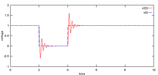
Step - 1/s
Ex)
|
Input
|
sys = tf([1],[1 0]) % Create a transfer function based on numerator and denominator
step(sys);
|
|
Output
|
Transfer function 'sys' from input 'u1' to output ...
1
y1: -
s
Continuous-time model.
|
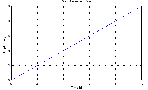
Step - 1/(a*s+1)
Ex)
|
Input
|
tau = 0.5;
sys = tf([1],[tau 1])
step(sys,5.0);
|
|
Output
|
Transfer function 'sys' from input 'u1' to output ...
1
y1: ---------
0.5 s + 1
Continuous-time model.
|
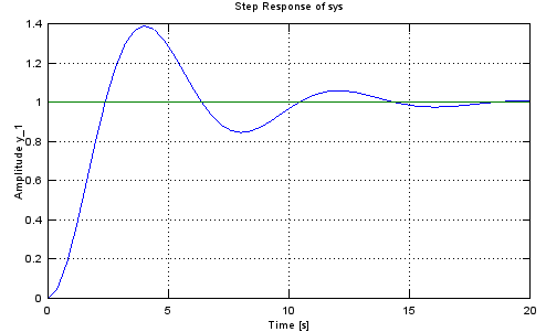
Step - 1/(a*s^2+b*s+1)
Ex)
|
Input
|
a = 1.5;
b = 0.7;
sys = tf([1],[a b 1])
step(sys,20.0);
|
|
Output
|
Transfer function 'sys' from input 'u1' to output ...
1
y1: -------------------
1.5 s^2 + 0.7 s + 1
Continuous-time model.
|
|
|