As you see in the plot show below, to some point the ideal operation curve and real operation curve of an amplifier is almost identical (i.e, within linear operation region) but from a certain point the real output signal gets compressed and the real output start diverging from the ideal (linear) curve. If you measure the divergence (the difference between the ideal line and real curve) along the operation curve, you would hit a specific point where the difference between the linear line (ideal operation line) and the real operation curve become 1 dB. That point is called 1dB compression point. Along with IP3, this point is used as an indicator showing the degree of nonlinearity of an amplifier.

Let's keep one question in mind through this page: how hard can I drive an amplifier before its gain stops being a constant? The 1dB compression point, usually written P1dB, is the most common single answer to that question. The sections below read the plot, put numbers on the definition, connect it to IP3 and show how the number is measured and used.

• What Does the Compression Curve Show?
• How Is P1dB Written in Numbers?
• How Does P1dB Relate to IP3?
• How Is P1dB Measured and Used?

What Does the Compression Curve Show?

An ideal amplifier multiplies every input by the same gain. So its output rises in a straight line as the input rises. A real amplifier follows that line only while the input is small. At some input level the transistor runs out of voltage or current swing, and the output grows more slowly than the input.

The plot below draws both behaviours on the same axes. The blue line is the ideal output and the red curve is the real output. The vertical line marks the input where the red curve starts to bend away from the blue line. Further up, a short arrow marks the input where the gap between the two has grown to 1 dB.

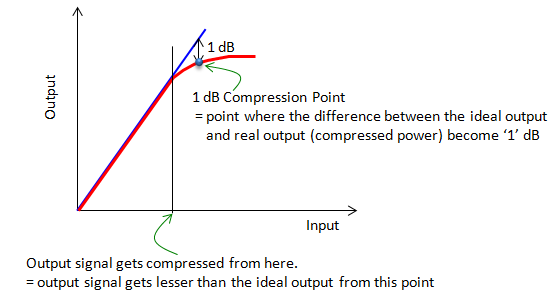
The real output falls below the ideal line gradually, not at one point. P1dB is the agreed place on that bend where the shortfall reaches 1 dB.

• The blue line is the linear gain : its slope is the small-signal gain. On dB axes the ideal line has a slope of 1, so 1 dB more input gives 1 dB more output.
• The red curve is what the amplifier really delivers : it lies on the blue line at low input, bends near the vertical marker and then flattens toward the saturated output power.
• The 1 dB arrow is measured vertically : it is the difference between the ideal output and the real output at the same input. The label in the plot calls this the compressed power.
• Compression starts well before P1dB : the note at the bottom of the plot says the output is already smaller than the ideal from the vertical marker on. P1dB does not mark the start of nonlinearity. It marks a level of nonlinearity that is easy to measure.

How Is P1dB Written in Numbers?

P1dB is a point on a curve, so it has two coordinates. A data sheet usually quotes only one of them, and you need to know which one before comparing two amplifiers.

Let's write the gain at input power P_in as G(P_in) in dB, and the small-signal gain as G₀. The compression point is the input power where G(P_in) = G₀ - 1 dB. That input power is the input-referred compression point, IP1dB. The output power at the same point is the output-referred compression point, OP1dB. The two are tied by a single relation.

OP1dB = IP1dB + G₀ - 1, with all terms in dBm or dB.

The -1 is easy to forget, because the gain at the compression point is no longer G₀. For example, an amplifier with G₀ = 20 dB and IP1dB = 0 dBm has OP1dB = 0 + 20 - 1 = 19 dBm, not 20 dBm. Receivers and mixers are usually specified by IP1dB, because the question there is how strong a signal the input can take. Power amplifiers are usually specified by OP1dB, because the question there is how much power they can deliver.

A simple model shows where the bend comes from. Write the amplifier as y = a₁x + a₃x³, with a₃ of opposite sign to a₁. For a sine wave of amplitude A, the cubic term adds (3/4)a₃A³ at the fundamental frequency. That term subtracts from a₁A, so the gain falls as A grows. Setting the fall to 1 dB gives A_1dB = √(0.145 x |a₁/a₃|). The 0.145 is (4/3) x (1 - 10^-1/20).

• P1dB always needs a reference : check whether a quoted value is input-referred or output-referred. For the same device the two differ by G₀ - 1 dB.
• The gain at P1dB is G₀ - 1 : so OP1dB is 1 dB below what the small-signal gain alone would predict.
• Compression comes from the odd-order terms : in the cubic model, a negative a₃ makes the output at the fundamental grow more slowly than a₁A.

How Does P1dB Relate to IP3?

Both P1dB and IP3 describe the same nonlinearity, as the opening paragraph says. So it is natural to ask whether one predicts the other. For the cubic model it does, and the gap has a fixed value.

In the cubic model, the input amplitude at the third-order intercept is A_IP3 = √((4/3) x |a₁/a₃|). Divide it by A_1dB from the previous section and convert to dB. The result is 20log₁₀(A_IP3/A_1dB) = 9.64 dB. The same model gives a compact formula for the gain at any input power, G(P_in) = G₀ + 20log₁₀(1 - P_in/P_IIP3), with both powers in linear units. The table below applies it to an amplifier with G₀ = 20 dB and IIP3 = +10 dBm.

The last row is the compression point. IP1dB is +0.36 dBm, which is 9.64 dB below IIP3, and OP1dB is 0.36 + 20 - 1 = 19.36 dBm. Notice how slowly the compression builds. It is below 0.1 dB until the input is 20 dB below IIP3, and it reaches 0.5 dB only about 3 dB before P1dB.

Real amplifiers do not follow the cubic model exactly. Fifth-order and higher terms, bias shifts and memory effects all change the shape of the curve near compression. So the 9.64 dB gap is a model result, not a data-sheet rule. When both numbers matter, use the measured IP3 and the measured P1dB. The IP3 page covers the intercept point itself.

• The cubic model puts IIP3 9.64 dB above IP1dB : this follows from 20log₁₀(A_IP3/A_1dB) and holds only when the third-order term dominates.
• IP3 is an extrapolation and P1dB is an operating point : an amplifier never reaches its intercept point. It does reach P1dB, which is why P1dB can be measured directly.
• Compression below P1dB is not zero : in the example, the gain is already 0.28 dB low at -5 dBm, about 5 dB below IP1dB. Measurements that need a very accurate gain have to stay further back.

How Is P1dB Measured and Used?

The definition turns directly into a measurement. You sweep the input power in small steps and record the gain at each step. The compression point is the step where the gain has dropped 1 dB below its small-signal value.

A signal generator and a power meter are enough for a single frequency. A network analyzer with a power sweep does the same job faster, and it can repeat the sweep across a frequency range. Three details affect the result. The first is the small-signal gain reference. It has to be taken at an input level low enough that the gain no longer changes when the input changes. The second is the step size near compression, which has to be fine enough to interpolate the 1 dB point. The third is heating. A power amplifier driven near compression warms up, and a slow sweep and a fast sweep can give different answers.

In a transmitter, P1dB sets how far back the average power has to stay. A modulated signal has a peak-to-average power ratio, PAPR, and its peaks reach the compression region first. If the peaks are compressed, the signal spreads into the neighbouring channels and the modulation accuracy drops. The ACLR/ACPR page measures that spreading. As a first estimate, keep the peaks near or below OP1dB. For example, an amplifier with OP1dB = +30 dBm and a signal with a PAPR of 8 dB gives an average output of about +22 dBm. The exact back-off depends on how much distortion the system can accept, so the final value comes from an ACLR and EVM measurement rather than from this estimate.

• P1dB is measured on a power sweep : record the gain at each input level and find where it is 1 dB below the small-signal gain.
• The gain reference must come from the linear region : if the reference level is already slightly compressed, the measured P1dB comes out too high.
• Back-off trades efficiency for linearity : an amplifier is most efficient near compression, but a signal with a high PAPR has to run its average power well below P1dB.