Techslide | ShareTechnote

Channel Matrix Example

The example shows the application of Singular Value Decomposition (SVD) to reveal the fundamental properties of a channel matrix in a communications system, likely a MIMO system. The illustration explicates this process and provides additional numerical insights into the channel characteristics.

This analytical approach using SVD offers valuable insight into the channel's properties and its influence on signal transmission, which is essential for designing communication systems that are both resilient and effective. The numerical data associated with the SVD provides a deeper understanding of the channel quality and its characteristics, enabling the implementation of signal processing techniques to refine transmission for better clarity and reliability.

Followings are the breakdown of the illustration :

Channel Matrix: The channel's effects on the transmitted signals are encapsulated in the matrix. The variable 'a' in this matrix applies only to the second layer and affect the gain of the second antenna.
SVD Decomposition of Channel Matrix: The channel matrix is broken down via SVD into three matrices:
- A left singular matrix,
- A diagonal matrix with singular values (which denote the channel's response strength across various directions),
- And a conjugate transpose of the right singular matrix.
The SVD is crucial for comprehending how the channel modifies different signal vectors, and the singular values depict the gains or losses in these directions.
Fundamental Characteristics of the Channel Matrix:
- Rank : The rank of a matrix indicates the number of linearly independent rows or columns. In the context of a MIMO system, it can imply the number of uncorrelated transmission paths available for data signals. A full rank indicates maximum spatial multiplexing benefits.
- Condition Number : The condition number gives an indication of the numerical stability of a matrix. A condition number close to one suggests that the matrix is stable and inversions or solutions to systems of equations using this matrix will be accurate and not prone to numerical errors.
- Determinant : The determinant of a matrix in signal processing often relates to the scaling factor of the signal space. A determinant of one means that the signal space's volume is preserved during transformation, indicating no net amplification or attenuation caused by the matrix. When the determinant of a matrix used in MIMO systems is a complex number, it suggests that the channel effects include a phase shift. In physical terms, not only is the signal potentially amplified or attenuated (as indicated by the magnitude of the determinant), but it is also rotated in the complex plane, which corresponds to a timing shift in the time domain. This phase shift must be accounted for in signal processing to ensure accurate signal reconstruction at the receiver. A complex determinant isn't uncommon in channels that have multipath propagation where different signal paths can interfere constructively or destructively, changing both the amplitude and phase of the received signal.
Transmitted and Received Data:Tx(1) and Tx(2): These charts display the data designated for transmission through the channel, depicted for two transmission layers or streams.H: This signifies the channel matrix's application to the transmitted data.
- Rx(1) and Rx(2): Post-channel transmission, the data is exhibited in these plots. The displacement of points from their original locations due to the channel is evident.

Followings are the code that I wrote in Octave to creates all the plots shown in this page. You may copy these code and play with these codes. Change variables and try yourself until you get your own intuitive understanding.

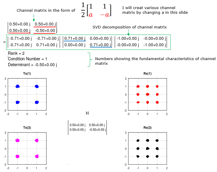
< Code 1 >

n = 0;

w = n * pi/40;

a = 0.5;

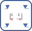
e11 = 1 + j*0;

e12 = a*exp(j * w);

e21 = a*exp(-j * w);

e22 = 1 + j*0;

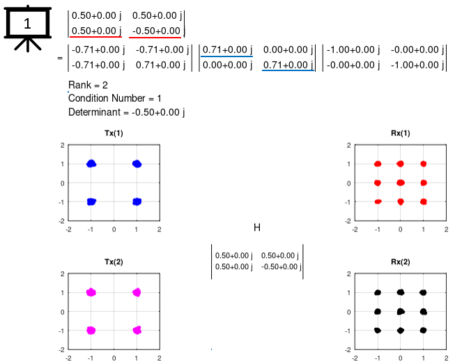
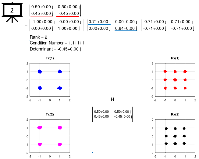
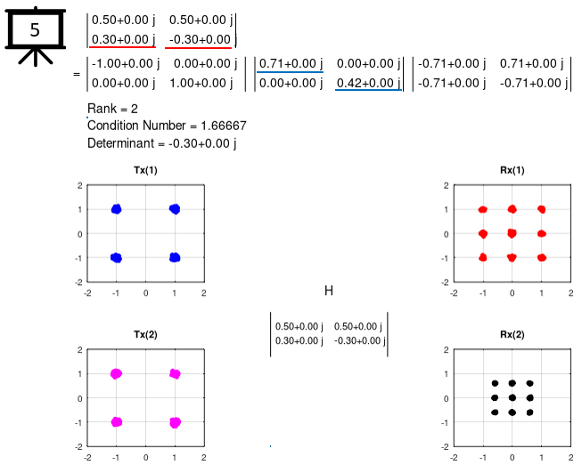
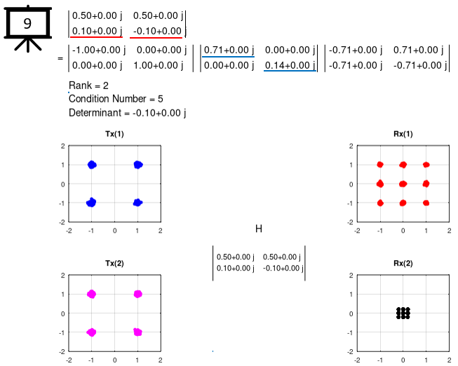
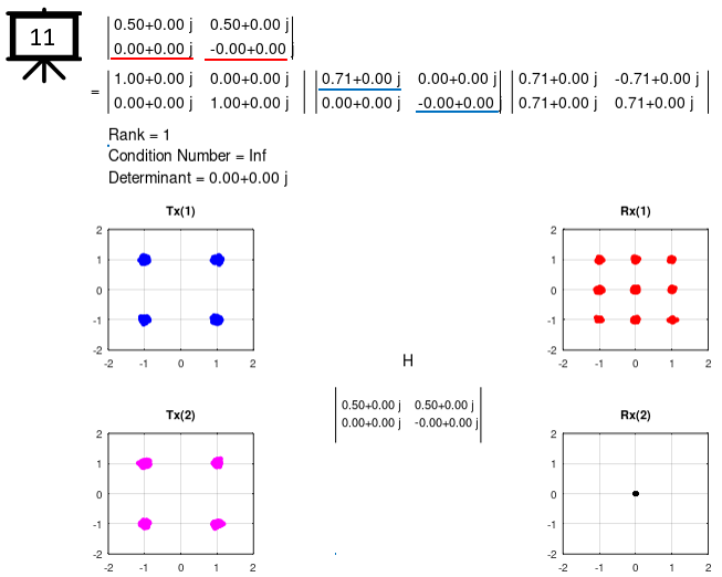
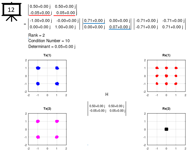
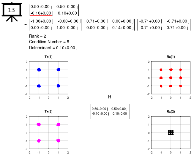
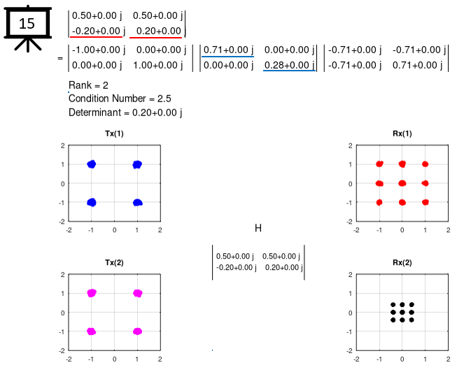
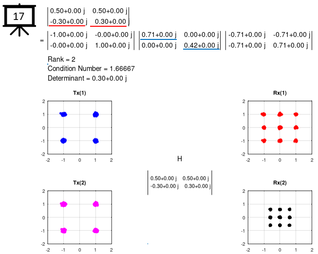
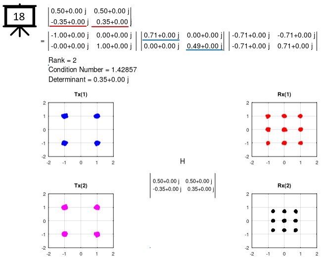
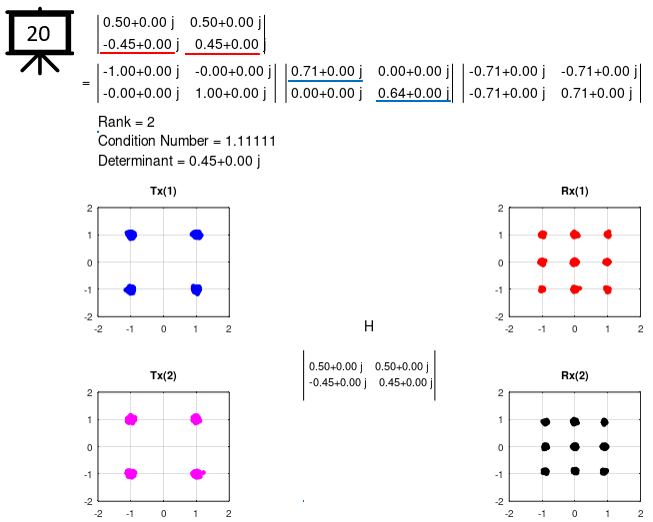
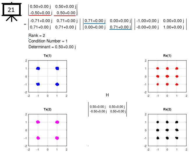
H = 1/(sqrt(2)) * [e11 e12;e21 e22];

[u, s, v] = svd(H);

r = rank(H);

c = cond(H);

d = det(H)

hFig = figure(1,'Position',[300 300 700 600]);

% ======================= Printing Matrix Information =========================

subplot(3,3,[1 3]);

hold on;

plot([0.0],[0.0]);

x0 = 0.01;

y0 = 0.0;

tStr = sprintf('%0.02f%+-0.02f j %0.02f%+-0.02f j\n%0.02f%+-0.02f j %0.02f%+-0.02f j', ...

real(H(1,1)),imag(H(1,1)),real(H(1,2)),imag(H(1,2)),...

real(H(2,1)),imag(H(2,1)),real(H(2,2)),imag(H(2,2)));

text(x0+0.0,y0+1.0,tStr,'FontSize',14,'color','black');

line([x0-0.01 x0-0.01],[y0+0.8 y0+1.2],'LineWidth',1,'Color','black');

line([x0+0.31 x0+0.31],[y0+0.8 y0+1.2],'LineWidth',1,'Color','black');

x0 = 0.01;

y0 = -0.2;

text(x0-0.04,y0+0.69,"=",'FontSize',14,'color','black');

tStr = sprintf('%0.02f%+-0.02f j %0.02f%+-0.02f j\n%0.02f%+-0.02f j %0.02f%+-0.02f j', ...

real(u(1,1)),imag(u(1,1)),real(u(1,2)),imag(u(1,2)),...

real(u(2,1)),imag(u(2,1)),real(u(2,2)),imag(u(2,2)));

text(x0+0.0,y0+0.7,tStr,'FontSize',14,'color','black');

line([x0-0.01 x0-0.01],[y0+0.5 y0+0.9],'LineWidth',1,'Color','black');

line([x0+0.32 x0+0.32],[y0+0.5 y0+0.9],'LineWidth',1,'Color','black');

tStr = sprintf('%0.02f%+-0.02f j %0.02f%+-0.02f j\n%0.02f%+-0.02f j %0.02f%+-0.02f j', ...

real(s(1,1)),imag(s(1,1)),real(s(1,2)),imag(s(1,2)),...

real(s(2,1)),imag(s(2,1)),real(s(2,2)),imag(s(2,2)));

text(x0+0.35,y0+0.7,tStr,'FontSize',14,'color','black');

line([x0+0.34 x0+0.34],[y0+0.5 y0+0.9],'LineWidth',1,'Color','black');

line([x0+0.65 x0+0.65],[y0+0.5 y0+0.9],'LineWidth',1,'Color','black');

tStr = sprintf('%0.02f%+-0.02f j %0.02f%+-0.02f j\n%0.02f%+-0.02f j %0.02f%+-0.02f j', ...

real(v(1,1)),imag(v(1,1)),real(v(1,2)),imag(v(1,2)),...

real(v(2,1)),imag(v(2,1)),real(v(2,2)),imag(v(2,2)));

text(x0+0.68,y0+0.7,tStr,'FontSize',14,'color','black');

line([x0+0.67 x0+0.67],[y0+0.5 y0+0.9],'LineWidth',1,'Color','black');

line([x0+1.00 x0+1.00],[y0+0.5 y0+0.9],'LineWidth',1,'Color','black');

tStr = sprintf('Rank = %d',r);

text(x0-0.01,y0+0.32,tStr,'FontSize',14,'color','black');

tStr = sprintf('Condition Number = %d',c);

text(x0-0.01,y0+0.12,tStr,'FontSize',14,'color','black');

tStr = sprintf('Determinant = %0.02f%+-0.02f j',real(d),imag(d));

text(x0-0.01,y0-0.1,tStr,'FontSize',14,'color','black');

axis([0.0 1.01 0 1.2]);

set(gca,'Visible','off');

hold off;

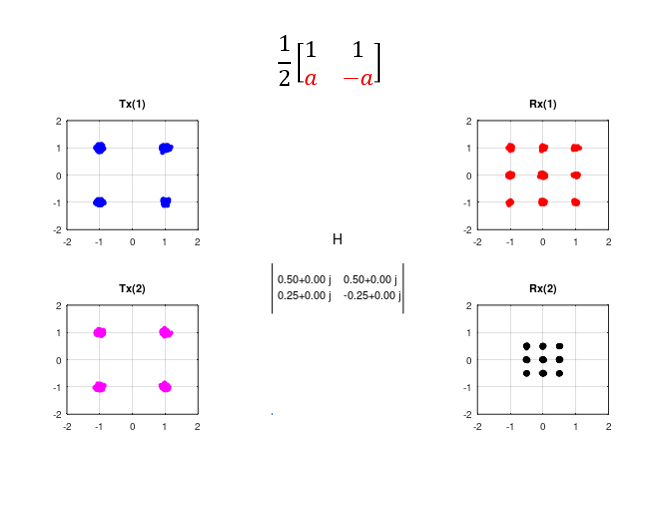
% ======================= Plot Constellation =========================

N = 500;

rand ("seed", 100);

n1 = 0.05*(randn(1,N) + j*randn(1,N));

n2 = 0.05*(randn(1,N) + j*randn(1,N));

c1 = (2*randi([0 1],1,N)-1) + j*(2*randi([0 1],1,N)-1);

c2 = (2*randi([0 1],1,N)-1) + j*(2*randi([0 1],1,N)-1);

c1 = c1 + n1;

c2 = c2 + n2;

n = 1;

Tx = [c1; c2];

Rx = H * Tx;

subplot(3,3,4);

plot(real(Tx(1,:)),imag(Tx(1,:)),'bo','MarkerFaceColor',[0 0 1],'MarkerSize',4);

axis([-2 2 -2 2]);

title('Tx(1)');

grid on;

box on;

subplot(3,3,7);

plot(real(Tx(2,:)),imag(Tx(2,:)),'mo','MarkerFaceColor',[1 0 1],'MarkerSize',4);

axis([-2 2 -2 2]);

title('Tx(2)');

grid on;

box on;

subplot(3,3,6);

hold on;

plot(real(Rx(1,:)),imag(Rx(1,:)),'ro','MarkerFaceColor',[1 0 0],'MarkerSize',4);

axis([-2 2 -2 2]);

title('Rx(1)');

hold off;

grid on;

box on;

subplot(3,3,9);

hold on;

plot(real(Rx(2,:)),imag(Rx(2,:)),'ko','MarkerFaceColor',[0 0 0],'MarkerSize',4);

axis([-2 2 -2 2]);

title('Rx(2)');

hold off;

grid on;

box on;

subplot(3,3,[5 8]);

hold on;

plot([0.0],[0.0]);

x0 = 0.1;

y0 = 0.0;

text(x0+1.0,y0+1.4,"H",'FontSize',14,'color','black');

tStr = sprintf('%0.02f%+-0.02f j %0.02f%+-0.02f j\n%0.02f%+-0.02f j %0.02f%+-0.02f j', ...

real(H(1,1)),imag(H(1,1)),real(H(1,2)),imag(H(1,2)),...

real(H(2,1)),imag(H(2,1)),real(H(2,2)),imag(H(2,2)));

text(x0+0.0,y0+1.0,tStr,'FontSize',11,'color','black');

line([x0-0.1 x0-0.1],[y0+0.8 y0+1.2],'LineWidth',1,'Color','black');

line([x0+2.28 x0+2.28],[y0+0.8 y0+1.2],'LineWidth',1,'Color','black');

axis([0.0 2.4 0 2.4]);

set(gca,'Visible','off');

hold off;