Neural Network -  Pereceptron - AND Logic

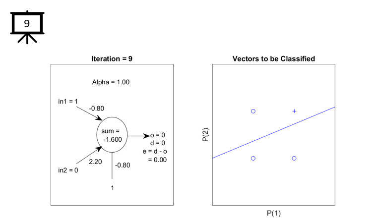
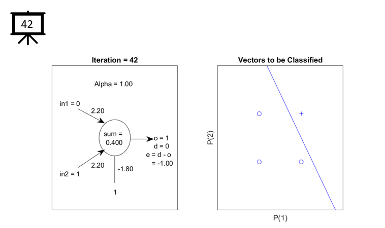
Followings are the code that I wrote in Deep Learning Toolbox (2019b)  to creates all the plots shown in this page. You may copy these code and play with these codes. Change variables and try yourself until you get your own intuitive understanding.

< Code 1 >

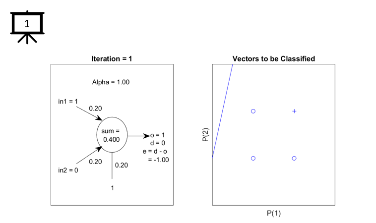
net = perceptron;

net = configure(net,[0;0],0);

net.b{1} =  [0.2];

w = [0.2 0.2];

net.IW{1,1} = w;

alpha = 1.0;

pList = [1 1 0 0; 1 0 1 0];

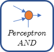
tList = [1 0 0 0]; % AND

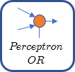
%tList = [1 1 1 0]; % OR

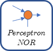
%tList = [0 0 0 1]; % NOR

figure(1);

set(gcf, 'Position', [200, 200, 740, 350])

set(gcf,'color','w');

subplot(1,2,2);

plotpv(pList,tList);

rng(1);

sList = randi([1 4],[1,100]);

for i = 1:60

    si = sList(i);

    p = pList(:,si);

    t = tList(si);

     a = net(p);

    %------------------------------------

    subplot(1,2,1);

    th = 0:pi/20:2*pi;

    plot(4+cos(th),4+sin(th),'k-');

    axis([0,8,0,8]);

    set(gca,'xticklabel',[]);

    set(gca,'yticklabel',[]);

    set(gca,'xtick',[]);

    set(gca,'ytick',[]);

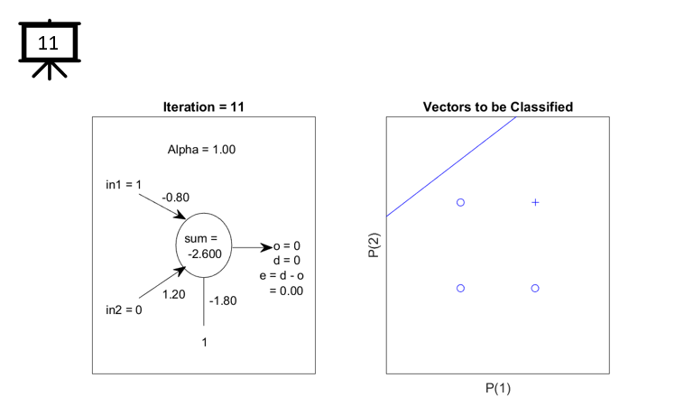
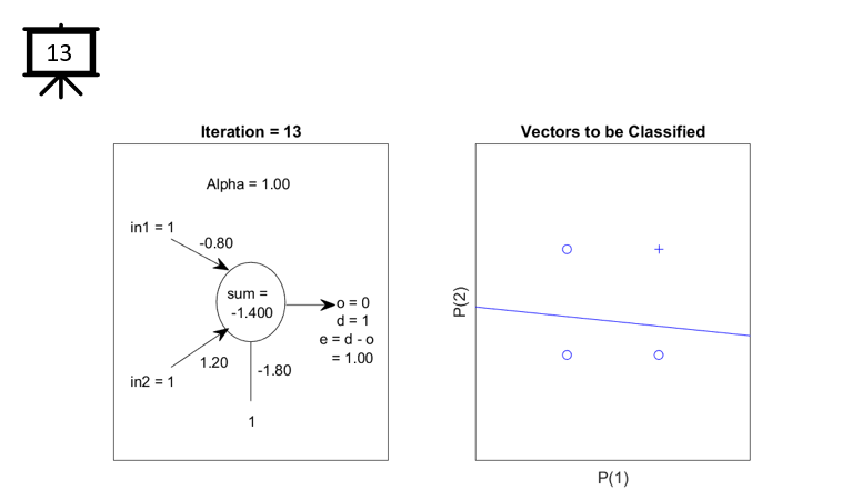
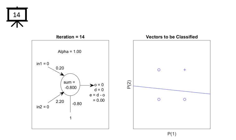
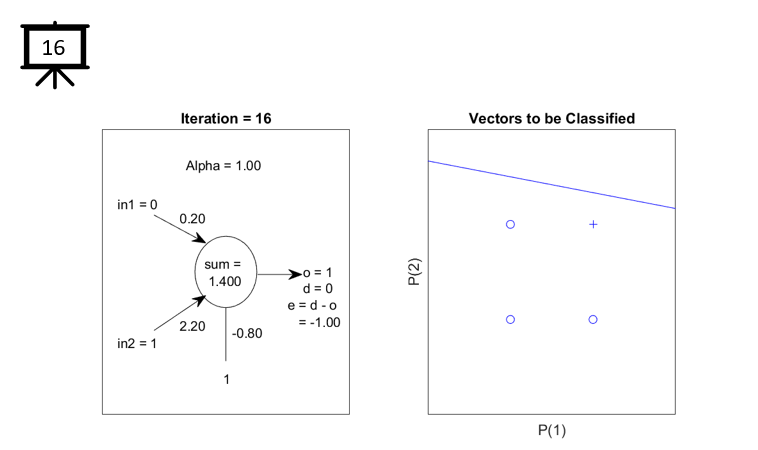
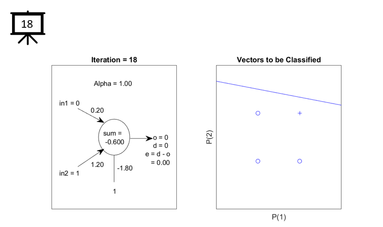
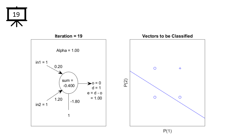
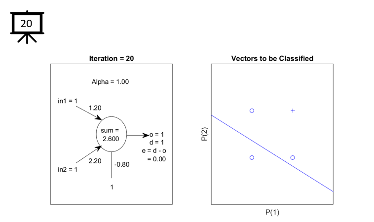
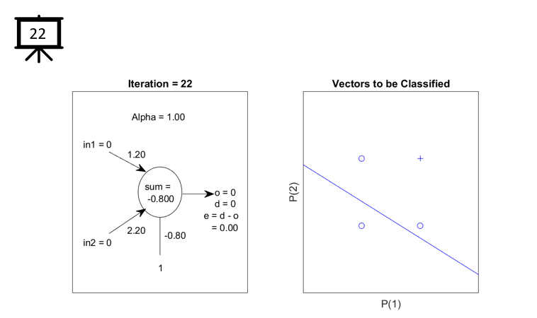
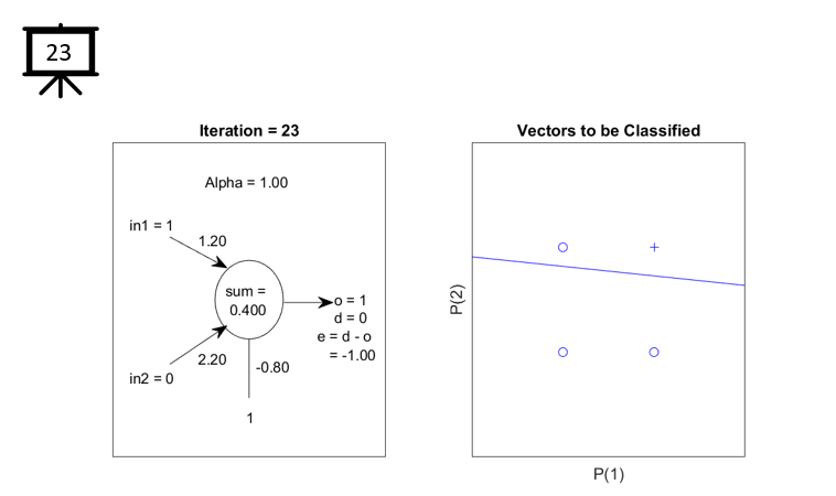
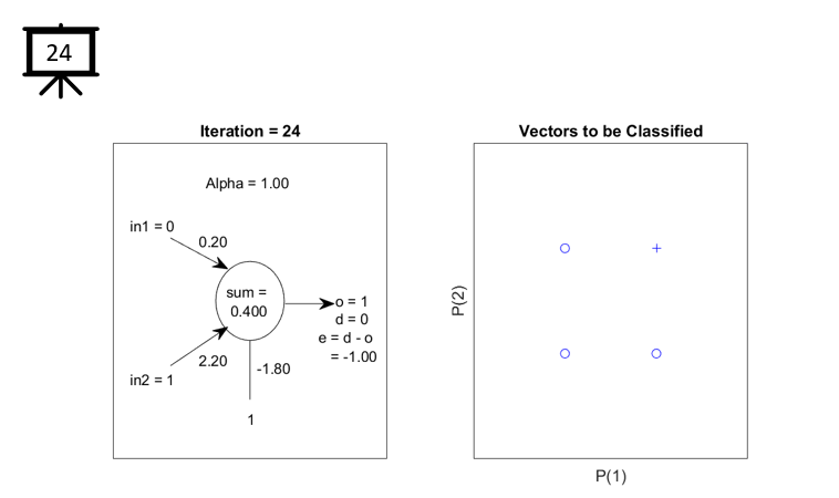
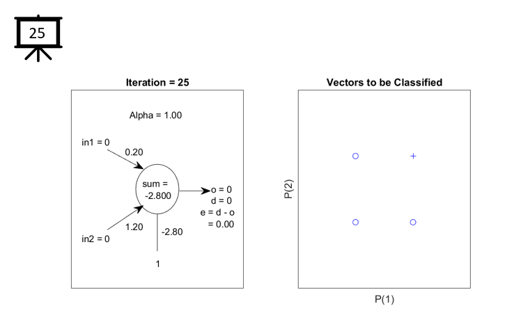
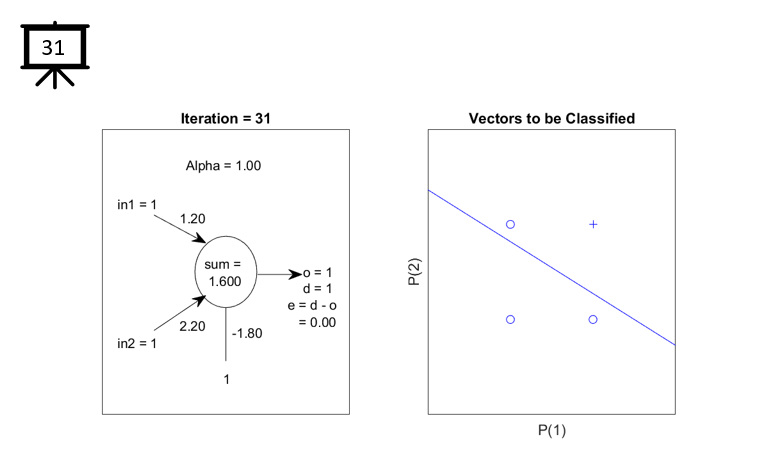
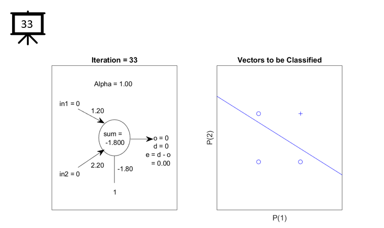
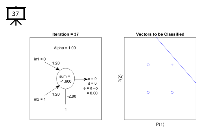
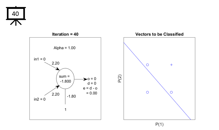
    tStr = sprintf("Iteration = %d",i);

    title(tStr);

    w1_ax = [0.2 0.27];

    w1_ay = [0.68 0.6];

    annotation('textarrow',w1_ax,w1_ay,'String','');

    w2_ax = [0.2 0.27];

    w2_ay = [0.35 0.45];

    annotation('textarrow',w2_ax,w2_ay,'String','');

    b_x = [4 4];

    b_y = [1.5 3];

    line(b_x,b_y,'color','black');

    o_ax = [0.34 0.4];

    o_ay = [0.51 0.51];

    annotation('textarrow',o_ax,o_ay,'String','');

    alphaStr = sprintf("Alpha = %0.2f",alpha);

    text(2.7,7.0,alphaStr);

    in1 = p(1);

    inStr1 = sprintf("in1 = %d",in1);

    text(0.5,5.9,inStr1);

    in2 = p(2);

    inStr2 = sprintf("in2 = %d",in2);

    text(0.5,2.0,inStr2);

    bStr = sprintf("1");

    text(3.9,1.0,bStr);

    b=net.b{1};

    bStr = sprintf("%0.2f",b);

    text(4.2,2.3,bStr);

    w1 = net.IW{1,1}(1);

    w1Str = sprintf("%0.2f",w1);

    text(2.5,5.5,w1Str);

    w2 = net.IW{1,1}(2);

    w1Str = sprintf("%0.2f",w2);

    text(2.5,2.5,w1Str);

    s = in1*w1 + in2*w2 + b;

    sStr = sprintf("sum = \n %0.3f",s);

    text(3.3,4,sStr);

    o = a;

    oStr = sprintf("o = %d",o);

    text(6.5,4.0,oStr);

    d = t;

    dStr = sprintf("d = %d",d);

    text(6.5,3.55,dStr);

    e = d-o;

    eStr = sprintf("e = d - o \n   = %0.2f",e);

    text(6.0,2.85,eStr);

    %------------------------------------

    subplot(1,2,2);

    plotpv(pList,tList);

    axis([-1 2 -1 2]);

    set(gca,'xticklabel',[]);

    set(gca,'yticklabel',[]);

    set(gca,'xtick',[]);

    set(gca,'ytick',[]);

    fprintf("\n----------- %d th iternation ---------------\n",i);

    fprintf("[%d %d] => %d\n",p(1),p(2),t(1));

    %a = net(p);

    fprintf("a = %f\n",a);

    e = t-a;

    fprintf("e = %f\n",e);    

    dw = learnp(w,p,[],[],[],[],e,[],[],[],[],[]);

    fprintf("dw = [%f %f]\n",dw(1),dw(2));

    net.b{1} = net.b{1} + alpha*e;

    w = w + alpha*dw;

    fprintf("w next = [%f %f], b next = %f\n",w(1),w(2),net.b{1});

    net.IW{1,1} = w;

    plotpc(net.IW{1,1},net.b{1});

    pause(1);

    fname = sprintf("%s/temp/PerceptronNOR_%02d.png",pwd,i);

    %saveas(gcf,fname);

end;

fprintf("\n----------- Evaluate the Net ---------------\n");

net(pList)