Tx diversity is the other special case of the generalized channel model. Rx diversity sets t = 1 and hands the receiver several copies to combine. Tx diversity sets r = 1 instead, so the transmitter holds several antennas and the receiver has a single antenna to listen on. That swap changes the problem completely, and most of this page explains why.

• The model : t Tx antennas and one Rx antenna
• Why the receiver cannot combine here
• Getting the diversity without knowing the channel

The model : t Tx antennas and one Rx antenna

Start from the same generalized r-by-t model and set r = 1 rather than t = 1. The received signal drops from a vector to a single value, and the channel matrix drops to a single row. The two equations below hold the whole model.

The expanded form comes first, so that the shape of every term stays visible, and the compact form follows it.

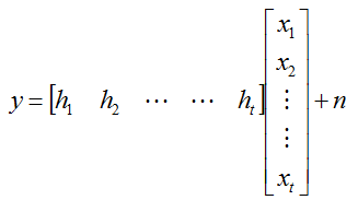
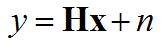
• y is one value rather than a vector, because the receiver has one antenna. The noise term n is a single value for the same reason.
• The channel is the row [h₁ h₂ ... h_t]. Each h_i is the coefficient of the path from Tx antenna i to that one Rx antenna.
• x is a column of t entries, one symbol per transmit antenna, exactly as in the generalized model.
• The compact form is the same y = Hx + n used everywhere else on this site. Only the dimensions have changed, with H now 1 by t.

Writing the product out gives y = h₁ x₁ + h₂ x₂ + ... + h_t x_t + n. Every symbol the transmitter sends arrives added into one number. The receiver therefore holds one measurement and t unknowns, and it cannot separate them. That single fact is the whole difficulty of Tx diversity, and the section below works through what follows from it.

Why the receiver cannot combine here

The Rx diversity page ends with a weight vector w and a rule for choosing it. Nothing of that kind is available here. The weighting has to happen before the signal is transmitted, and the transmitter is the end that knows least about the channel.

Compare the two cases directly. With one Tx antenna and r Rx antennas, the receiver holds r separate measurements y₁ to y_r, and it also holds an estimate of h from its own channel estimation. It can therefore choose w after seeing both, and Maximal Ratio Combining is that choice. With t Tx antennas and one Rx antenna, the receiver holds one measurement and can choose nothing.

Moving the weighting to the transmitter raises two problems at once. The transmitter does not measure the downlink channel, so it does not know h. The transmitter also has to apply the weights before the symbol leaves, which is before the receiver has seen anything at all. Feedback closes that gap, and the closed loop schemes on the SVD page do exactly that with a PMI report.

Feedback costs something, though. It costs uplink capacity for the report itself, and it costs accuracy whenever the channel changes between the measurement and the transmission that uses it. A scheme is therefore worth having if it needs no feedback at all, even when it gives up part of the gain.

A second problem appears here that the Rx case never meets. Sending one symbol from every transmit antenna gives no diversity. The copies add at the single receive antenna as h₁ x + h₂ x + ... + h_t x, which is x multiplied by the sum of the coefficients. That sum can be small while the individual coefficients are not, so the deep fades remain. They have only changed where they occur.

Getting the diversity without knowing the channel

The answer is to spread each symbol across the transmit antennas and across time, rather than across the antennas alone. Two symbol periods then give the receiver two measurements, and two measurements are enough to solve for two unknowns.

Alamouti coding is the two antenna case, and every standard that uses transmit diversity starts from it. Over the first symbol period antenna 1 sends s₁ and antenna 2 sends s₂. Over the second period antenna 1 sends the negated conjugate of s₂ and antenna 2 sends the conjugate of s₁. The receiver collects y over both periods and recovers both symbols.

The orthogonality of those two transmissions is what makes it work. The two columns the receiver ends up with are orthogonal, so separating s₁ from s₂ costs a conjugate and an addition rather than a matrix inversion. The full derivation sits on the Alamouti Code/OSTBC page.

The diversity order matches Rx diversity, and the cost differs. Alamouti needs no channel knowledge at the transmitter and no feedback, so it still works on a fast channel where a PMI report would already be stale. It does need h₁ and h₂ to stay constant across the two symbol periods. It also gives about 3 dB less than two receive antennas would, because the transmit power is split across two antennas while a second receive antenna collects extra energy.

• Tx diversity is the r = 1 case of the generalized model, so the channel matrix H is the single row [h₁ h₂ ... h_t].
• The receiver gets one measurement for t transmitted symbols, so it cannot combine the way an Rx diversity receiver does.
• Sending one symbol from every antenna gives no diversity. It replaces each coefficient with the sum of them all.
• Closed loop schemes solve this with feedback, at the cost of uplink capacity and of accuracy on a fast channel.
• Alamouti coding solves it with no feedback, by spreading two symbols over two antennas and two symbol periods.