This page derives zero forcing one branch at a time, rather than as a single matrix inversion. The derivation follows what happens to symbol x_k on its own, and it separates the received energy, the cross-talk from the other symbols, and the noise. Reading it that way makes the cost of zero forcing visible as a term in an equation rather than as a general warning.

This page (knowledge) is shared by James Weng who is a real expert in this area.

• The MIMO system model and noise whitening
• Combining the receive antennas
• Forcing the cross-talk to zero
• The price paid in noise

The MIMO system model and noise whitening

Everything that follows rests on one equation and one assumption. The equation is the linear MIMO model. The assumption is that the noise is white, with a normalized covariance matrix. Whitening is the step that makes the assumption true when a real channel does not deliver it, and that is why it appears this early rather than as a footnote.

Consider an MIMO system with  m-Tx antennas and  n-Rx antennas. A received signal vector from  -Rx antennas can be written into this form,

where y is the received signal vector and  z is a noise vector and they both are with dimension  n x 1, H  is an MIMO channel matrix with dimension n x m , and x  is an  m x 1 column vector for m transmitted symbols.

Given the received signal vector y  and assuming the channel matrix H  is known, our goal is to detect x .

For the detection, we further assume the noise vector  z is a white Gaussian with zero-mean and a normalized co-variance matrix  E{zz^H} = I . For the cases where the noise vector is not white, i.e., the co-variance matrix  E{zz^H} = Rzz , we then need to whiten the noise first by multiplying (Rzz)^-1/2 first to both sides of equation (1). We have,

Note that equation (2) is the same as equation (1) if we absorb the noise whitening matrix (Rzz)^-1/2 into the channel matrix H and consider the received signal vector and the noise vector are the ones after the noise whitening operation. Therefore, here, for the sake of simplicity, we assume the noise has been whitened and we use equation (1) to further explain how to detect (or estimate) the symbol vector x.

Combining the receive antennas

Now, back to equation (1), to combine the received symbol replicas from multiple receive antennas, we often multiply H^H  to both sides of the equation to yield,

It is interesting to note that the diagonal elements of the channel matrix  (H^H H) combine the energy of each symbol replica from the receive antennas. To be specific, the  k-th element of (H^H y) can be expressed into this form

where  h_ij is the ij-th entry of the MIMO channel matrix H.

The first term at the right hand-side of the above equation is a combined energy of symbol replicas of x_k from all receive antennas, the second-term is actually interference, representing cross-talks from other symbols, and the third-term is for noise.

Often, we do a further normalization by dividing the above by the gain 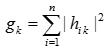to yield a decision variable for symbol x_k . The decision variable can be written as

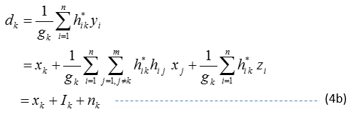
, where

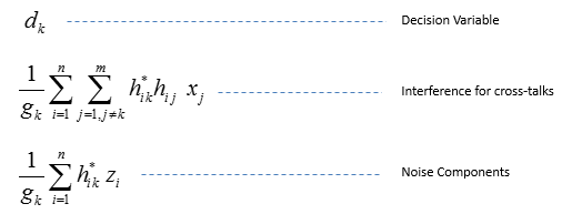
Obviously, if there is no cross-talk, equation (4) means a maximal ratio combining to form a decision variable d_k for symbol  x_k. If x_k  is QAM symbol , we can estimate x_k  by checking which QAM decision region that d_k falls into.

Forcing the cross-talk to zero

In the presence of cross-talks, the maximal ratio combining might not be a good detection approach for symbol x_k. We have heard of the zero-forcing approach, which basically tries to force the cross-talk to 0 by multiplying the inverse of (H^H H) to both sides of equation (3), i.e.,

For notational simplicity, we denote W = (H^H H)^-1  as the weighting matrix for the zero-forcing and we re-employ d = H^H y  as the decision vector before the zero-forcing operation. Equation (5) can be rewritten as

and its  k-th element can be expressed as

where

Equation (6) holds the whole of zero forcing in one line. The left side is what the receiver computes, and the right side splits into the transmitted vector and a noise term. No interference term survives the multiplication by W, which is exactly what the name promises.

Equation (7) says the same thing for one symbol. The left side is a weighted sum of the decision variables d_j across all m branches, with the weights w_kj taken from row k of W. The right side is x_k plus one noise term. Reaching x_k therefore costs a sum over the branches, and every branch in that sum brings its own noise along with its signal.

One index in the last equation above needs care. The label reads j-th elements in noise vector, and the sum on the right is written with h^*_ik. The subscript should follow j rather than k, because the expression gives the j-th entry of (H^H z).

The price paid in noise

If we compare equation (7) and equation (4b), we can infer that the zero-forcing does some weighting and combining of decision variables  d_j from other branches, i.e., (j <> k) , in order to remove the interference term I_k. That type of weighting and combining of decision variables obviously will bring noises from other branches into this k-th branch for symbol x_k. In other words, the noise component in Equation (7)  will be larger than the noise component in (4b) as a result of forcing the interference term  I_k in (4b) to 0 by combining the decision variables from other branches. Basically, if we use (4b) as the decision variable for symbol  , we will suffer from the interference  . If we zero-force the interference to 0 by using (7) as the decision variable, the resulting noise in (7) will be larger than the original noise in (4b).

How much larger depends on W, and W is the inverse of (H^H H). When the columns of H are nearly parallel, that matrix comes close to singular, its inverse holds large entries, and the weights w_kj that multiply the other branches grow with them. Noise from those branches then arrives at branch k scaled up rather than scaled down.

This is the effect that the main Zero Forcing page calls noise amplification, seen one branch at a time instead of through the covariance matrix. The two derivations reach the same conclusion. Zero forcing buys a clean interference term and pays for it in noise, and the size of the payment is set by the conditioning of H.

Equation (4b) and equation (7) therefore mark the two ends of a choice. Take (4b), keep the smaller noise, and live with the interference I_k. Take (7), remove I_k, and accept the larger noise. MMSE sits between the two, because it weighs the interference against the noise variance instead of removing either one outright.