What is BeamForming ? It means just as it sounds. BeamForming is a technology to 'Form' a 'beam'.
Then what does it mean by 'beam' in this context ? I would say it means 'electromagnatic wave radiation pattern(propagation pattern) for a set of antenna system'. Simply put, BeamForming is a technique that constructs the antenna radiation pattern pointing towards specific direction.
One point is worth making clear from the very beginning, because it is the source of most of the confusion around this topic.
Before diving into the details, let me give you 'super simplified' principles of beamforming/beamsteering.
1. If you put multiple number of antenna with a certain distances, you will always have some special shape of beam which is different from the radiation pattern from single isotropic antenna.
2. if you want to have a specific shape of beam you need to put those multiple antenna in a specific distances between them ==> BeamForming
3. if you want to point the beam toward a specific direction, you need to transmit the signal through each of the antenna elements with certain amount of phase difference. ==> BeamSteering
It is worth noticing the difference between item 2 and item 3 in the list above, because these two are decided at completely different moments in the life of a system.
The geometry (item 1 and item 2) - how many elements there are and how far apart they sit - is fixed at the moment the antenna is manufactured. You cannot change it while the network is running. It decides theshape of the beam : how narrow it can possibly be, and how strong the unwanted side lobes are.The phase (and amplitude) applied to each element (item 3) is just a number in a register, or a control voltage. It can be changed within microseconds. It decides thedirection of the beam.
This is exactly why a base station can sweep a beam across a whole sector many times per second without any moving part. Nothing rotates. Only numbers change.
High level meaning is simple like this.. but real implementation would be very complicated and is out of my understanding. So I would just give you only a big picture of this technology.
- Motivation (Why we need BeamForming ?)
- High Level view of BeamForming Implementation - Mapping Function, Spatial Filter
- How to 'Form' a beam ?
- Technology for BeamForming
- Basic Concept : Array Antenna
- Characterization of Array Antenna - Beam Pattern Plot
- Basic Concept : Beam Forming - Phased Array
- Modeling BeamForming
- Beamforming in LTE
- Precoding for BeamForming
- Single-layer random beamforming (Antenna port 5, 7, or 8) : 36.101 B.4.1
- Dual-layer random beamforming (antenna ports 7 and 8) : 36.101 B.4.2
- Generic beamforming model (antenna ports 7-14) : 36.101 B.4.3
- Example 1 : 8 x 2 (8 Antenna, 2 Layers)
- CSI RS Configuration
- Beamforming in 5G/NR (Massive MIMO)
Motivation (Why we need BeamForming ?)
Why we need beamforming ?
It is simple. Let's look at the two illustrations as shown below. There are two antenna system and let's assume that the two antenna is transmitting the exactly same amount of total energy.
In case 1, the antenna system is radiating the energy in almost same amount in all direction. The three UEs around the antenna would receive almost same amount of the energy but a large portions of energy not directed to those UEs is wasted.
In case 2, the signal strength of the radiation pattern ('beam') is specially 'formed' in such a way that the radiated energy in direction to UEs are much stronger than the other parts which is not directed to UEs.
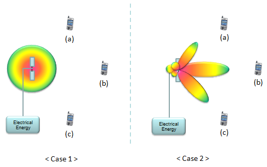
A few details in this illustration are worth a closer look.
- The box labelled 'Electrical Energy' is the
same in both cases. This is the point I made in the introduction : no extra power is being supplied. The pattern on the right is simply the same energy arranged differently in space. - In Case 2 the pattern has
three lobes, one pointing at each of the three UEs, and not a single pencil beam. A beam pattern does not have to be one single lobe. As long as the phases are chosen correctly, one array can put energy into several directions at the same time. - Look at the small lobes pointing backwards and sideways in Case 2. Those are the
side lobes , and they never completely disappear. Some part of the energy always leaks into directions you did not ask for.
There is also a second benefit which this picture does not show directly, but which matters just as much in a real network. In Case 1, the energy that is 'wasted' does not simply vanish - it flies into the neighbouring cells and becomes
And the same argument works in the uplink as well, only in the opposite direction. A receiving array that 'listens' in a narrow direction collects more of the wanted signal and less of the noise and interference that arrives from all the other directions.
High Level view of BeamForming Implementation - Mapping Function, Spatial Filter
Very high level view on how to implement BeamForming can be illustrated as follows. It shows a set of data is going into a special function and the special function form a specific beam and transmit the data through the beam. The shape and direction of a beam is determined by what kind of function is used. This kind of special function is often called as BeamForming Function or Mapping Function or Spatial Filter. Applying the same Mapping function or Spatial Filter mean that it forms the same beam (i.e, same direction, same shape, same power of the beam).

Take a moment to compare the four panels in this illustration, because the message is in what stays the same and what changes.
- The
hardware is identical in all four panels : the same number of antenna elements, in the same positions. - The
input data is identical as well. The same d0, d1, ... d(n-1) go into the box in every panel. - The only thing that changes is the function inside the box : F1, F2, F3, F4. And as a result, a different lobe out of the fan of possible beams becomes the strong one (drawn as a solid orange lobe) while all the others stay weak.
So the whole of beamforming, seen from outside, is this :
You may also notice that the thin fan of lobes is drawn in every panel. This is meant to show the set of beams that this array is
Now the question is how these mapping function (or beamform algorithm) is implemented. The remaining of this page is all about the general logic of this mapping function. Simply put, the major component of the mapping functions are
- Number of Antenna Elements in the array
- Structure of Antenna Elements in the array
- Phase and Amplitude applied to each of the data(signal) path => this can be done in software at the baseband or hardware(electrical circuit) at RF or mmWave frequency
How to 'Form' a beam ?
By now, you would ask 'How can we form a beam ?'. If you want to understand this mechanism in precise and clear way, you need to turn to the dry and boring mathematics. We will look into this mathematical way of explanation in following section (Basic Concept : Array Antenna), but before falling asleep with math, let's build up some intuitive understanding on the principles of the beam forming.
The basic principle of forming a beam is to use the property of interference of the multiple waves. If the multiple waves interfere each other at 'In-phase', the amplitude of the interfered waves gets bigger (this is called 'Constructive interference). If the multiple waves interfere each other at 'Out-of-phase', the amplitude of the interfered waves cancels each other(this is called destructive interference). If multiple waves propagating in 2D or 3D spaces, the resulting interference would show a specific pattern in which some part of the spaces shows constructive interference and some other parts shows destructive interference. The part performing constructive interference form a beam pointing to a specific direction. Check out this slides(animation) and hope you can get some intuitive understanding.
The simplest way of forming a beam is to put multiple antenna in an array. There are many different ways of aligning those antenna elements, but one of the simplest way is to align the antenna along a line as shown in the following example. The intuitive idea you should see here is that you will get a sharper beam as you put more antenna elements in the array.
Also I have posted several pages in my visual note : www.freetechslide.com in the form of slideshow and animations of various antenna radiation pattern so that you can understand the radiation pattern for various antenna structure in more intuitive way. Check [Engineering]->[1]->[Antenna Radiation], [Array Antenna] in www.freetechslide.com

Look at the four plots (A) to (D) above and count the blue dots, which are the antenna elements.
(A) : with only a couple of elements the beam already exists, but it is very wide and there is nothing else to see.(B) : with more elements the main lobe is clearly narrower, and small side lobes have appeared beside it.(C) and (D) : as the element count keeps growing, the main lobe keeps getting narrower and the side lobes keep multiplying.
Two rules of thumb come out of this single picture, and they are worth memorizing because they hold for every array you will ever meet.
Doubling the number of elements roughly halves the width of the main lobe. More elements = sharper beam. What actually matters is the total physical length of the array (the aperture) measured in wavelengths.More elements also means more side lobes. They become thinner as they multiply, but they never go away. Side lobes are the price you pay for directivity, and keeping them under control is a large part of real antenna design (see the amplitude weights w1 ... w8 in the Phased Array section below).
Another way of arranging the elements in an array is align the elements in a two dimensional square as shown in the following examples. The intuitive idea you should see here is that you will get a sharper beam as you put more antenna elements in the array.

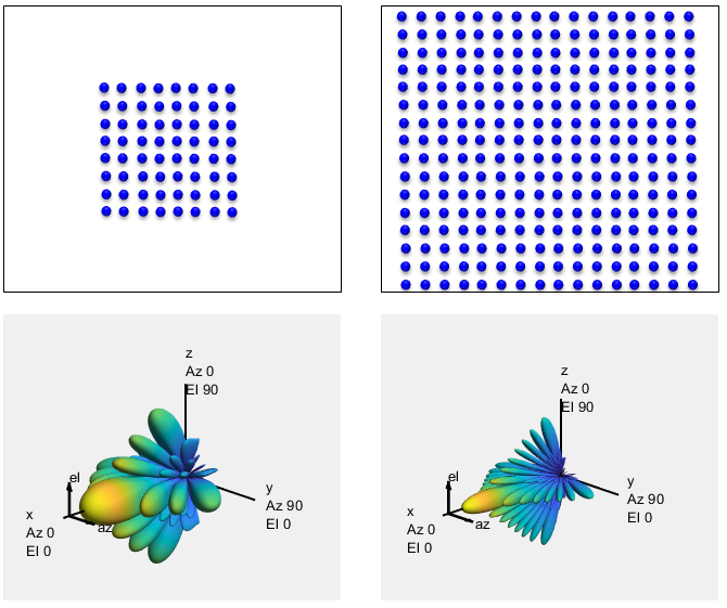
The step from a line to a plane is not only about making the beam sharper. A linear array can steer in
In 3GPP language this is exactly what makes FD-MIMO (Full Dimension MIMO) and vertical sectorisation possible : the network can aim one beam at the 3rd floor of a building and a different beam at the 20th floor of the building next to it. It is also why the element count grows so fast - an 8 element line becomes an 8 x 8 = 64 element plane, and planar arrays of roughly this size are what commercial massive MIMO products are built from.
Now let's think of another type of two dimensional array in which the shape of the array is not square as shown below. The intuition you can get is that the beam compressed more along the axis of more elements.

This last pair of plots is probably the most practical one of the four, because a real base station antenna is almost never square. Notice how each pattern is 'squeezed' in the plane where the array is long, and stays wide in the plane where the array is short. A tall, narrow array gives a beam that is narrow in elevation and wide in azimuth ; a short, wide array does the opposite.
This is exactly how an ordinary sector antenna is built. It is a tall, narrow column of elements, because a base station wants a beam that is wide enough to cover a 120 degree sector horizontally, but narrow vertically so that the energy is aimed down at the street rather than up into the sky. So the long thin shape of the antenna you see on any tower is not an accident of packaging - it is the beam pattern requirement made visible.
Technology for BeamForming
There are several different ways to implement the beamforming. Followings are couple of techniques most commonly used (As I mentioned, the details of implementation is out of my understanding).
For a little bit further details, see All Beamforming Solutions Are Not Equal. This is mainly for WLAN, but can be a good introduction.
- TM 6 - Closed loop spatial multiplexing using a single transmission layer.
- TM 7 - Beamforming (Antenna port 5)
- TM 8 - Dual Layer Beamforming (Antenna ports 7 and 8)
- TM 9 - Up to 8 layer transmission (Antenna ports 7 to 14) with CSI-RS based feedback. This is the transmission mode used in the 8 x 2 example later on this page.
- TM 10 - The same port set as TM9 (ports 7 to 14), extended for CoMP (Coordinated Multi Point), i.e, more than one transmission point is involved.
The three techniques listed above are not really competitors of each other. They sit at different places in the transmit chain, and a real product very often uses more than one of them at the same time.
Switched array antenna is the crudest and the cheapest. There is no phase control at all, only a set of fixed patterns that you select between. It is fast and simple, but the number of beams you can make is exactly the number of switch combinations that were built into the hardware.DSP based phase manipulation andbeamforming by precoding are in fact the same idea seen from two different angles. Both of them apply a complex weight (a phase and an amplitude) to every antenna path. The only real difference iswhere that weight is applied - in an analog RF circuit after the OFDM signal has been generated, or as a matrix multiplication in the baseband before it. This same distinction comes back as "Pure RF vs Pure Baseband vs Hybrid" in the LTE section below.
Basic Concept : Array Antenna
Since the BeamForming is mostly based on Array Antenna, let's take a look at the basic principles of Array Antenna. Let's suppose we have a antenna array in which each of the antenna is placed apart from each other with a certain distance (d). And then, suppose multiple rays of beam transmitted from a single source is received by each of the antenna in the array. If all the rays from the single source is coming directly (meaning theta in the following illustration is 0) into the antenna, there would be no differences in terms of distance along which each of the rays travelled from the source to each of the receiver antenna. So if you sum up the energy received by each antenna, it will be same as each of the wave sum up constructively. However, if the direction of the ray and the axis of antenna array is not in right angle (meaning the theta is not 0), the travel distance of each ray (p1,p2,..,p8) gets different and the difference can be expressed as d sin(theta) as shown in the following illustration.
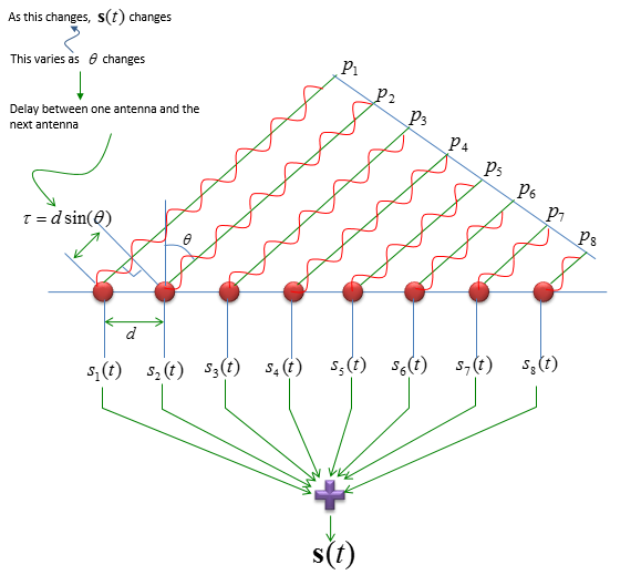
The single most important quantity in this whole picture is the little triangle drawn on the left,
- When
θ = 0 (the source is straight ahead, on the normal of the array), sin(θ) = 0 and therefore τ = 0. All eight paths then have exactly the same length, all eight signals arrive in phase, and the sum is as large as it can possibly be. This is the main lobe - and notice that it is therewhatever the spacing d happens to be. - As
θ grows, the eight signals arrive progressively out of step and begin to cancel each other in the sum. This is why the pattern falls off as you move away from the main lobe.
Note also that the path difference between one element and the next is always the same τ, so the phase difference builds up
Now let's describe what I explained above into mathematical expression. If I take the received signal at the first antenna (the leftmost antenna) as the reference antenna and the signal received at each of the antenna can be represented as follows. (This would the point where many people gave up further reading/study because of the math. But in most of engineering and science, there are many cases where you can never understand completely without a certain degree of math. So, don't give up just because of the math... and try to understand the meaning of each mathematical terms. When I am explaining about this array antenna, I first talked about the travel path difference and angle between antenna array axis and the beam ray hitting the antenna. In the mathematical expression, you still see the angle term 'theta', but you don't see any direct term that look like 'travel path'. Actually we don't know the exact travel difference of each beam because we don't know the exact location of the beam source. The only thing we know is the travel path difference between each beam hitting on each antenna. That travel path difference can be expressed as e^(-j * n * d * theta) where n is the index of the antenna being numbered 0 from the leftmost antenna. Keeping this in mind, take close look at each mathematical expression and it would make sense to you. If you are not familiar with interpreting the meaning of e^(-theta), you may refer to complex number page).
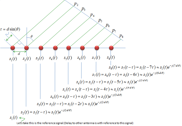
The fact that only the ratio d/λ matters has a very visible practical consequence. At 700 MHz a half wavelength is about 21 cm, so an 8 element array is well over a metre long. At 28 GHz a half wavelength is about 5 mm, so the same 8 elements fit into 4 cm. This is why an array with dozens of elements can be hidden inside a phone at mmWave, and it is the main reason why massive MIMO arrived together with the high frequency bands rather than before them.
Another way of visualizing this summation process would be as follows :
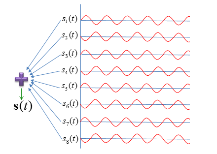
In this drawing each row is the signal arriving at one element, and you can see the waveforms slipping progressively sideways as you go down the list. That slipping is the phase ramp caused by τ being added one more time at every element. The summation on the left is then the whole story of the array in one symbol : whether the sum comes out big or small depends only on whether these eight waves happen to line up or not, and that in turn depends only on the arrival angle.
Now we formulated the signal coming into each antenna. Now let's formulate the signal that combined all the signal coming into each antenna. It is simple, you only have sum up all the signals comining into each antenna and it can be presented as follows.

You can represent this equation into a vector notation as follows.(Many people even including me get intimidated when seeing this kind of matrix/vector expression. Don't get scared. We have already learned basic operations from high school or freshmen university math course. We just didn't have enough chance for enough practice. So if you get somehow uneasy feeling about this, just expand the following equation by hand and you will get more familiar expression as above. Doing this kind of practice whenever you see this kind of vector/matrix notation, gradually you will get more and more familiar and such an uneasy feeling would disappear. Nobody else can do this kind of practice for you)

The vector a(θ) in this expression has a name of its own in the literature - it is called the
And this leads straight into the idea behind the next two sections. If a(θ) is the phase pattern that direction θ
Characterization of Array Antenna - Beam Pattern Plot
When you characterize (represent the performance of an Antenna array), you might have seen the types of plots as shown below. In some documents, you would see the plot like the one on the left and in some other document you would see the one on the right. Actually these two represents the exact the same thing. They just plot the same thing in two different coordinate system. The one on the left is the representation of (transmitted or received power) vs angle in Cartesian coordinate and the right one is the representation of the same data in polar coordinate.
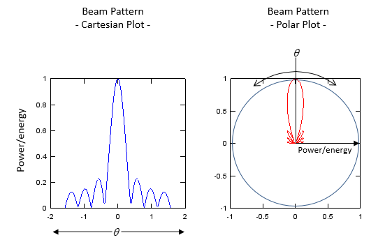
Both plots show exactly the same curve, and it is worth naming the features you can see in them, because these names turn up in every antenna datasheet.
Main lobe : the big peak in the middle. This is what everybody means by 'the beam'.Beamwidth : how wide the main lobe is. It is normally quoted as thehalf power beamwidth (HPBW), i.e, the angle between the two points where the power has fallen to half of the peak, which is 3 dB down.Side lobes : the smaller bumps on both sides of the main lobe. In the Cartesian plot on the left you can count them easily ; in the polar plot on the right they are the little petals around the base of the main beam.Nulls : the points between the lobes where the curve touches zero. These are directions the array is effectively deaf and blind to, and a clever system will deliberately steer a null toward a strong interferer.
Power and Energy in the plot would be familiar to you. Then, what does the theta (angle) represents ? It is the angle between the direction of ray and the
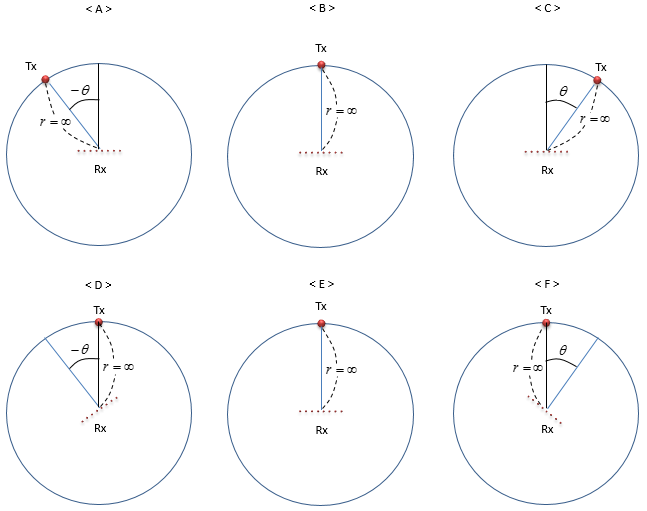
The same logic applies when the transmitter antenna is the array antenna and the receiver antenna is a point far away from the transmitter. The angle is, again, the angle between the direction of ray and the

In above illustration, you have seen four different cases of representing the angle. Even though the function of the antenna array (being receiver or transmitter) is different and the way making the angle (by moving receiver/transmitter antenna by rotating the antenna array), the overall shape of the plot is same (at least in theory). The only difference would be the scale of Energy/Power depending on whether it represents the receiver power or transmitter power. So if we ignore the scale of the engery/power axis, you can interpret the graph (Power/energy vs theta) as shown below.
As you see here, the energy/power gets maximum when the angle (theta) is 0.
- If the spacing is made
too large (roughly d ≥ λ), the phase difference between neighbouring elements can reach a whole turn at some other angle as well. At that angle the signals also add up perfectly, and a second, unwanted main lobe appears. This copy of the main beam is called agrating lobe , and it is a serious problem, because the array would be radiating full power into a direction that nobody asked for. - If the spacing is made
too small , the array becomes physically compact but the elements start to couple to each other electrically, and the beam gets wider for the same number of elements - because what really sets the beamwidth is the total size of the array (the aperture), not the element count on its own.
Half a wavelength is the compromise that avoids grating lobes across the whole steering range while keeping the array as small as possible. That is why you see λ/2 quoted everywhere.
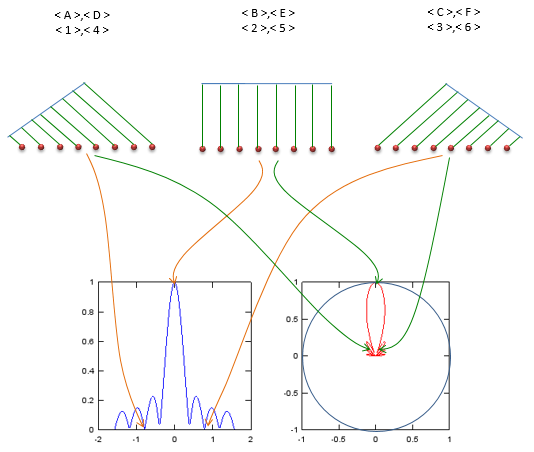
This last illustration ties the six sub plots together. The group in the middle (<B>,<E>,<2>,<5>) is the θ = 0 case : the wavefront reaches every element at the same instant, all the contributions add up, and this maps to the peak of the curve in both of the plots at the bottom. The groups on the left and on the right are the tilted cases, where the wavefront reaches the elements one after another, the contributions no longer line up, and the result maps to a point somewhere away from the peak.
What this really shows is that the beam pattern is
If you want to play with this graph, try running the follow matlab toy code.
theta = -0.5*pi:pi/100:0.5*pi;
d = 2.0;
a_theta = [exp(-j .* 0 .* d .* theta) ;
exp(-j .* 1 .* d .* theta);
exp(-j .* 2 .* d .* theta);
exp(-j .* 3 .* d .* theta);
exp(-j .* 4 .* d .* theta);
exp(-j .* 5 .* d .* theta);
exp(-j .* 6 .* d .* theta);
exp(-j .* 7 .* d .* theta)];
a_theta_sum = sum(a_theta);
a_theta_sum_abs = abs(a_theta_sum);
a_theta_sum_abs = a_theta_sum_abs ./ max(a_theta_sum_abs);
a_theta_sum_abs_dB = 20 .* log10(a_theta_sum_abs);
for i = 1:length(a_theta_sum_abs_dB)
if a_theta_sum_abs_dB(i) <= -30
a_theta_sum_abs_dB(i) = -30;
end;
end;
a_theta_sum_abs_dB = a_theta_sum_abs_dB - min(a_theta_sum_abs_dB);
a_theta_sum_abs_dB = a_theta_sum_abs_dB/max(a_theta_sum_abs_dB);
subplot(2,2,1);plot(theta,a_theta_sum_abs);
xlim([-pi/2 pi/2]);
set(gca,'xtick',[-pi/2 -pi/4 0 pi/4 pi/2]);
set(gca,'xticklabel',{'-pi/2' '-pi/4' '0' 'pi/4' 'pi/2'});
subplot(2,2,2);polar(theta + 0.5*pi,a_theta_sum_abs,'-r');
t = findall(gcf,'type','text');
delete(t);
subplot(2,2,3);plot(theta,20 .* log10(a_theta_sum_abs));ylim([-30 1]);
xlim([-pi/2 pi/2]);
set(gca,'xtick',[-pi/2 -pi/4 0 pi/4 pi/2]);
set(gca,'xticklabel',{'-pi/2' '-pi/4' '0' 'pi/4' 'pi/2'});
subplot(2,2,4);polar(theta + 0.5*pi,a_theta_sum_abs_dB,'-r');
t = findall(gcf,'type','text');
delete(t);
- The dB conversion. The earlier version of this snippet used
10 .* log(...) , which is wrong on two counts : in Matlablog is the natural logarithm (the base 10 one is log10), and the quantity being converted here is anamplitude , so the correct conversion is 20*log10(x) and not 10*log(x). It is corrected in the listing above. The dB traces in the plotted images on this page were produced with the earlier expression, so read their vertical scale as illustrative rather than calibrated - the shape of the curve is right, but the numbers are stretched by roughly a factor of 1.15. d = 2.0 in this code is not a distance in metres, and not in wavelengths either. Because the model uses the simplified exponent e^(-j n d theta) with the 2*pi/lambda factor folded away, d is simply a dimensionless knob controlling how fast the phase ramps across the array. Increasing it narrows the beam in the same way that making the array physically longer would.
By tweaking the phase of each antenna, you can create a beam pointing to multiple direction as shown the following example. (Upper track is the power/energy in linear scale and Lower track is the power/energy in dB scale)
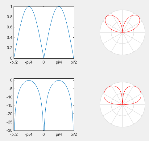
What the code does in order to achieve this is worth noticing. It builds two groups of four elements, one group driven with (theta - theta_shift) and the other with (theta + theta_shift), and then sums all eight. In other words the array has been split into two sub arrays, each of them steered to a different angle, and the resulting pattern therefore has two main lobes. This is the simplest possible example of what a real network does when it serves two users sitting in different directions from the same antenna at the same time.
The lower pair of plots is exactly the same data drawn on a dB scale. It is worth getting used to reading the dB version, because on a linear scale everything below about 10 percent of the peak simply looks like zero, while on a dB scale you can actually see how strong the side lobes are and how deep the nulls go. Antenna datasheets are almost always in dB for this reason.
Following is the matlab code for the plot shown above. Play with this by changing theta_shift or any other values in a_theta array as you like until you get the intuitive understanding of each parameters.
theta = -0.5*pi:pi/100:0.5*pi;
d = 2.0;
theta_shift = (0.25*pi);
a_theta = [exp(-j .* 0 .* d .* (theta-theta_shift));
exp(-j .* 1 .* d .* (theta-theta_shift));
exp(-j .* 2 .* d .* (theta-theta_shift));
exp(-j .* 3 .* d .* (theta-theta_shift));
exp(-j .* 0 .* d .* (theta+theta_shift));
exp(-j .* 1 .* d .* (theta+theta_shift));
exp(-j .* 2 .* d .* (theta+theta_shift));
exp(-j .* 3 .* d .* (theta+theta_shift))];
a_theta_sum = sum(a_theta);
a_theta_sum_abs = abs(a_theta_sum);
a_theta_sum_abs = a_theta_sum_abs ./ max(a_theta_sum_abs);
a_theta_sum_abs_dB = 20 .* log10(a_theta_sum_abs);
for i = 1:length(a_theta_sum_abs_dB)
if a_theta_sum_abs_dB(i) <= -30
a_theta_sum_abs_dB(i) = -30;
end;
end;
a_theta_sum_abs_dB = a_theta_sum_abs_dB - min(a_theta_sum_abs_dB);
a_theta_sum_abs_dB = a_theta_sum_abs_dB/max(a_theta_sum_abs_dB);
subplot(2,2,1);plot(theta,a_theta_sum_abs);
xlim([-pi/2 pi/2]);
set(gca,'xtick',[-pi/2 -pi/4 0 pi/4 pi/2]);
set(gca,'xticklabel',{'-pi/2' '-pi/4' '0' 'pi/4' 'pi/2'});
subplot(2,2,2);polar(theta + 0.5*pi,a_theta_sum_abs,'-r');
t = findall(gcf,'type','text');
delete(t);
subplot(2,2,3);plot(theta,20 .* log10(a_theta_sum_abs));ylim([-30 1]);
xlim([-pi/2 pi/2]);
set(gca,'xtick',[-pi/2 -pi/4 0 pi/4 pi/2]);
set(gca,'xticklabel',{'-pi/2' '-pi/4' '0' 'pi/4' 'pi/2'});
subplot(2,2,4);polar(theta + 0.5*pi,a_theta_sum_abs_dB,'-r');
t = findall(gcf,'type','text');
delete(t);
Basic Concept : Beam Forming - Phased Array
In previous sections on basic Antenna array model, we could see that just by arranging multiple antenna in an array we could create a beam with the directivity to a certain direction and by physically rotating the antenna array we can change the direction of the beam. However, there will be a lot of restrictions in terms of the shape of the beam and controlling the direction in simply placing multiple antenna in an array.
There are even smarter idea as invented as shown below. You can do everything explained above and do even more by placing the devices that can control phase and amplitude of a wave to each antenna as illustrated below.
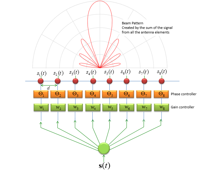
There are two separate rows of control blocks in this illustration and they do two different jobs. Mixing them up is a very common misunderstanding, so it is worth separating them clearly.
- The
phase controllers (Θ1 ... Θ8) decidewhere the beam points . Feeding a linearly increasing phase across the elements tilts the beam, and the bigger the step from one element to the next, the bigger the tilt. This is beam steering. - The
gain controllers (w1 ... w8) decidewhat the beam looks like . Giving every element the same weight produces the narrowest possible main lobe, but relatively strong side lobes. Giving more weight to the elements in the middle of the array and less to the ones at the edges - this is called amplitude tapering, or windowing - pushes the side lobes down a great deal, at the cost of a somewhat wider main lobe. It is the same trade off as windowing before an FFT, and for exactly the same mathematical reason.
So :
One more thing to notice in this drawing : there is only
The total energy pattern (beam pattern) created by summing up all the transmitted energy coming out of each antenna can be described in mathematical form as shown below.

Again, you can simplify this long equation into a simple vector notation as shown below. Theoretically, you can create a beam with any shape and any direction by changing the gain and phase in the vector.

Modeling of Beam Forming
As I mentioned above, theoretically you can create a beam with any shape and any angle by changing the angle (phase) and gain connected to each antenna. Then the question is how to find proper angle (phase) and gain value to each antenna to achieve the desired beam pattern.
Long story.. but the conclusion is not that complicated. Let's asume that we have the simplest array antenna made up of just two antenna as shown below. The antenna array on the left is transmitter antenna and the single antenna on the right is the receiver antenna. The blocks labeled p1 and p2 is a complex number that representing phase and amplitude controller (As you know, a complex number can represent both phase and amplitude). h1 and h2 is channel coefficient between transmitter and receiver antenna.
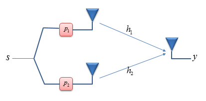
Now the question is how to represent the received signal y using these parameters. It can be presented as shown below (If you are not familiar with this kind of channel representation, refer to Channel Model page)

Now the question is how to find p1 and p2 value to make the beam properly point to the receiver antenna. If you rewrite the question a little bit, it can be 'what is the p1 and p2 value that maximize the received energy at the receiver antenna ?'. In real situation, h1 and h2 act as some factors distorting/deteriorating the signal between the transmitter and receiver antenna. So, if we can set p1 and p2 properly to compensate (line up) the phase rotation caused by h1 and h2, that would be the p value to make the received energy maximum. h1 and h2 are complex numbers, meaning h1 and h2 has gain component and phase component. Therefore, the question becomes 'how to undo an effect caused by a complex number ?'.
Undoing a complex number is simple. Just multiplying a complex conjugate to the given complex number. (If you multiply a complex number with its conjugate, the phase of the resulting complex number become always '0', meaning that imaginary part become always 0. So in this kind of situation, we can say 'multiplying a complex number with its conjugate' is same as 'undoing the phase shift caused by the complex number'.
Therefore, if you put complex conjugate of h1 and h2 into p1 and p2 as shown below, this would undo the phase shifting effect of h1 and h2.
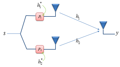
This looks very handy and simple solution. However, there is a problem with this kind of undo. By multiplying the channel coefficient with its conjugate, we can easily remove the phase part. However, the magnitude of the resulting number is changed as well (multiplying h by its conjugate gives |h| squared, not 1). To prevent this, you only have to normalize those conjugate numbers with the norm of h vector (a vector made of h1 and h2) as shown below.
Now with this, we found the p1 and p2 to make the beam in the best direction to the receiver antenna.
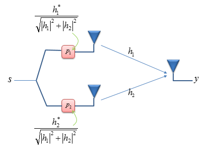
This result has a name that is worth knowing, because you will meet it constantly in MIMO literature. It is called
Two observations make this small formula much more meaningful than it first looks.
- The normalization is not a mathematical decoration. Without it, the transmitter would be asking for more power than it actually has. Dividing by the norm of h is what keeps the total transmit power constant - which brings us straight back to the point made at the very top of this page : beamforming redistributes power, it does not create it.
- The formula needs
h . Everything here depends on the transmitter knowing the channel, and that is the genuinely difficult part in a real system. There are only two ways to get it. Either the receiver measures it and sends it back - this is what PMI feedback does in LTE FDD, and it is the reason the whole codebook machinery described further down this page exists - or the system relies on channel reciprocity in TDD and measures the uplink instead, which is what SRS based beamforming does. Almost everything that follows in the LTE section is, in the end, the story of how h is obtained and how it is squeezed into a few bits.
If you implement the p1 and p2 in DSP or FPGA, the illustration above is good enough. Because you can easily implement a complex number as it is. However, if we implement p1 and p2 as analog component, probably following illustration would be a better representation.

The reason for splitting the complex number into two separate blocks in this last drawing is purely a hardware one. A complex multiplication is trivial in a DSP or an FPGA, but in the analog domain there is no such thing as 'multiplying by a complex number' - there is a phase shifter, and there is a variable gain amplifier, and they are two different physical components. So the same p1 is implemented as the
Beamforming in LTE
Overall procedure for LTE beamforming in the context of physical layer processing goes as shown below.
< Precoding for BeamForming >
In case of BeamForming, Precoding is doing almost nothing and instead something similar to Precoding happens at the stage labeled as BF(Beam Forming) shown below. Theoretically we can implement Beamforming in roughly three different way as illustrated below. But as far as I understand, in LTE < Case 1 > is most commonly used. (NOTE : in the system which use a lot of antenna as in 5G/NR, it is mostly likely to use < Case 3 > )
< Case 1 : Pure Baseband >
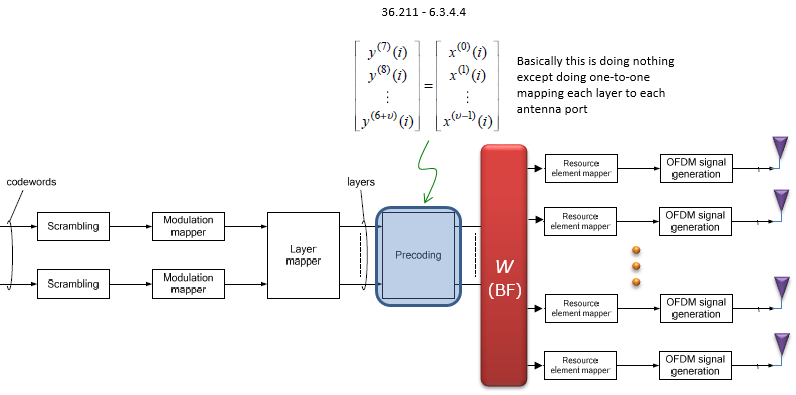
In this case the beamforming matrix W sits
Basic Beamforming Model for this type is described in 36.101 (B.4.1, B.4.2, B.4.3) and it proposes three different categories as summarized below. (Those three categories are the three sub sections that follow, after the remaining two implementation cases have been illustrated.)
< Case 2 : Pure RF >
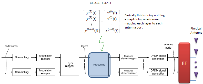
Here the picture is the opposite. The OFDM signal is generated first, and the beam is formed
< Case 3 : Hybrid >
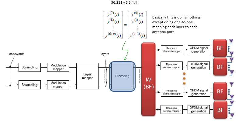
The hybrid case is the compromise, and it is the one that actually got built in 5G. A small number of transmit chains (in NR these are called TXRUs) feed a baseband matrix W, and each of those chains then drives a whole sub array of elements through its own bank of analog phase shifters. You end up with a manageable number of digital chains while still lighting up hundreds of physical elements. The digital part provides the multi user and multi layer flexibility ; the analog part provides the aperture and the gain.
A useful way to keep the three cases straight is to ask where the border between 'numbers' and 'metal' is drawn.
Pure Baseband : all of the beamforming is done in numbers. Most flexible, most expensive, does not scale to huge arrays.Pure RF : all of the beamforming is done in metal. Cheapest, scales well, least flexible.Hybrid : the coarse beam is made in metal, the fine adjustment is made in numbers.
- These models come from
36.101 Annex B , which is the UEradio conformance test specification. They are not a description of how a commercial eNB decides its beams. They are a definition of what a piece of test equipment has to transmit, so that every UE on the market is tested against the same, repeatable beamformed signal. - That is also where the word
random comes from. The test model deliberately picks the precoder at random out of the codebook and keeps changing it, so that the UE cannot 'learn' the beam and has to demodulate it purely from the reference signal it is given. In a real network the precoder is of course not random at all - it is chosen from the PMI report, or from uplink measurements.
So read the next three sections as "what a beamformed signal looks like", and not as "how a beam is chosen".
< Single-layer random beamforming (Antenna port 5, 7, or 8) : 36.101 B.4.1>
This type has following two cases. TM8, DCI Format 2B single layer would fall into this type.
i) without a simultaneous transmission on the other antenna port

ii) with a simultaneous transmission on the other antenna port

The difference between the two cases above is easy to miss in the formulas. In case i) only one of the two UE specific ports is active, so a single vector W(i), taken from the rank-1 column of the codebook, is applied to that one port. In case ii) port 7 and port 8 are both carrying data at the same time - either two layers to the same UE, or one layer each to two different UEs in MU-MIMO - so two independently chosen vectors W1(i) and W2(i) are applied and the results are summed, with the 1/√2 factor keeping the total transmit power unchanged.
< Dual-layer random beamforming (antenna ports 7 and 8) : 36.101 B.4.2>
TM8, DCI Format 2B dual layer would fall into this type.
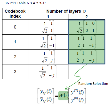
Notice that the highlighted column of the codebook has moved. Here it is the rank-2 column that is being used, so W(i) is a 2 x 2 matrix rather than a 2 x 1 vector, and it maps the two layers y(7) and y(8) onto the two antenna ports together. This is the dual layer case : the array is now carrying two independent data streams, so it is genuinely doing beamforming and spatial multiplexing at the same time.
< Generic beamforming model (antenna ports 7-14) : 36.101 B.4.3 >
TM9, DCI Format 2C dual layer would fall into this type.

The generic model is the one that scales, and the illustration tells you its shape directly. W(i) is a matrix with
Unlike other model like B.4.1 and B.4.2, the definition of W(i) is not always obvious. The 36.101 B.4.3 says "The precoder matrix W(i) is specific to a test case.", it means we have to define a specific test case (situation) and then try to define the W(i).
Example 1 : 8 x 2 (8 Antenna, 2 Layers)
In this example, I will look into a case where two layered data is transmitted through 8 Tx antenna. Two UE specific reference signal p7, p8 are subject to BeamForming and 8 CSI RS ports (p15~p22) will be transmitted for CSI estimation on UE side. Overall mapping between antenna ports and physical antenna is as shown below.
< Mapping between Antenna port and physical antenna >
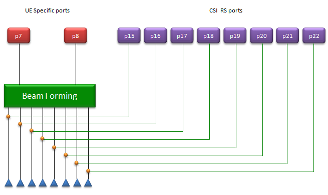
This illustration is worth spending a minute on, because it shows the two very different roles that antenna ports play here, and this is the heart of how LTE beamforming actually works.
- The two red ports on the left,
p7 and p8 , are the UE specific ports. They carry the two data layers together with their reference signal, and they gothrough the Beam Forming block, so what comes out is spread over all eight physical antennas. The UE measures the channel of p7 and p8 and therefore measures the beam and the propagation channel together, as one single thing. The UE never has to know what W(i) was. - The eight purple ports on the right,
p15 to p22 , are the CSI-RS ports. Look carefully at the drawing : theybypass the Beam Forming block completely and connect straight to the eight physical antennas, one to one. This is deliberate. Their job is to let the UE see the eight raw antennas separately, so that it can work out which precoder would be the best one and report it back as PMI.
So the two sets of ports form a loop. CSI-RS goes out
First, it seems obvious that we need something to distribute the two layered data over 8 physical antenna and it can be easily understood that we need following form of matrix.
< Beamforming Matrix converting two user ports to 8 physical antenna >

Reading the dimensions straight off this picture : the vector on the right has 2 entries (the two layers y(7) and y(8)), the vector on the left has 8 entries (one for each physical antenna, y_bf(0) through y_bf(7)), so W(i) has to be an
Now we have to figure out (or define) values of each matrix element. For this, we have to define our model more specifically.
36.213 7.2.4 Precoding Matrix Indicator (PMI) definition says as follows and this example is the case described by the underlined parts.
For transmission modes 4, 5 and 6, precoding feedback is used for channel dependent codebook based precoding and relies on UEs reporting precoding matrix indicator (PMI). For transmission mode 8, the UE shall report PMI if configured with PMI/RI reporting.
The exact value of the matrix is determined by UE PMI report and network construct the matrix W(i) based on following table.
36.213 Table 7.2.4-2 Codebook for 2-layer CSI reporting using antenna ports 15 to 22
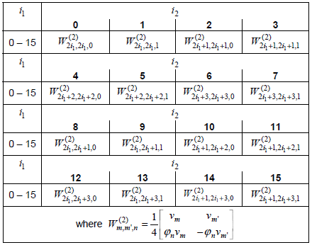
The first thing that confuses me was "Where is i_1 and i_2 is defined ?" and what do they mean (indicate) ? These are described in 36.213 section 7.2.1 "Wideband feedback -> Mode 1-2 description" as shown below. Of course it will take a long time to understand real meaning of these variable. (First you have to understand everything on CQI/RI Feedback type page first just to understand these i_1 and i_2)

The reason there are two indices instead of one is a very practical one, and it is a nice piece of engineering. For 8 antenna ports a single flat codebook would be far too large to report frequently, so the codebook is factorised into two parts.
i1 selects agroup of beams. It describes the slowly changing, wideband part of the channel - essentially the general direction the UE is sitting in - so it can be reported rarely and for the whole band at once.i2 selectsone beam within that group , and also the co-phasing between the two polarizations. This is the fast, frequency selective part, so it is reported more often and per sub-band.
This split is exactly what you can see in the structure of W(2) a little further down : the v_m term (which comes from i1) is the beam direction, and the φ_n term (which comes from i2) is the co-phasing between the two halves of the matrix. The very same 'two stage codebook' idea was carried forward into NR as the Type I codebook, so this is not just LTE trivia.
Following is more detailed information from 36.212 regarding the i1 and i2 report from UE.
< 36.212 - Table 5.2.3.3.1-3A: UCI fields for joint report of RI and i1 (transmission mode 9 configured with PMI/RI reporting with 2/4/8 antenna ports and transmission mode 10 configured with PMI/RI reporting with 2/4/8 antenna ports) >

< 36.212 - Table 5.2.3.3.2-2B: UCI fields for channel quality feedback for UE-selected sub-band reports (transmission mode 9 configured with PMI/RI reporting with 8 antenna ports and transmission mode 10 configured with PMI/RI reporting with 8 antenna ports) >
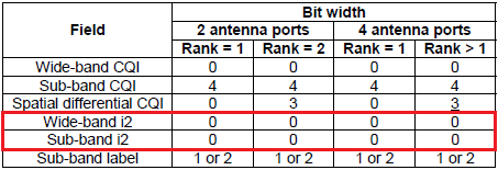
< 36.212 - Table 5.2.3.3.2-2B: UCI fields for channel quality feedback for UE-selected sub-band reports (transmission mode 9 configured with PMI/RI reporting with 8 antenna ports and transmission mode 10 configured with PMI/RI reporting with 8 antenna ports) >
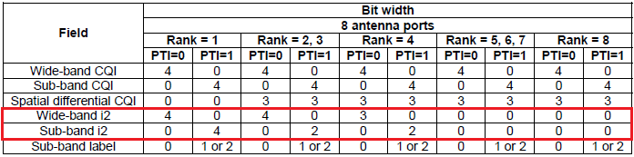
Now let's look into more details of W(i) matrix. Let's construct the generic form of W(i) matrix for this case. The matrix is defined at the bottom of the table shown above.
You would notice that W(i) is made up of following two components.
With Reference to 36.213 7.2.4

These two small definitions are the entire codebook. Read physically, they say :
v_m is a 4 element vector whose entries are equally spaced phase rotations (m, 2m, 3m in units of 2π/32). This is nothing other than the steering vector from the array antenna section at the top of this page, sampled at 32 possible directions. Choosing m is choosing where to point.φ_n = e^(jπn/2) takes only four values - 1, j, -1, -j, i.e, 0, 90, 180 and 270 degrees. This is the co-phasing term, and it exists because the 8 antennas of a typical LTE array are not 8 separate positions in space. They are 4 positions with two polarizations at each position. φ_n aligns the two polarizations with each other.
This is also why the 8 x 2 matrix in the next illustration is built out of 4 element blocks : v_m fills the four co-polarized elements, and φ_n v_m fills the four cross-polarized ones.
With the two components, you can construct the generic form of W(i) matrix as shown below. For each specific case, we have to figure out m, m' and n to fill out the matrix with specific values. and m, m' and n is determined by the PMI report and Table 7.2.4-2.
With Reference to 36.213 Table 7.2.4-2

And notice the last detail in this matrix : the second column uses
The 1/4 in front is the power normalization. The matrix has 16 entries, each of magnitude 1, so dividing by 4 brings the total transmitted power back to 1 - the same 'do not create energy' rule that has been showing up on every step of this page.
< CSI RS Configuration >
As described above, the key issue of Beamforming implementation is how to figure out proper BeamForming matrix for each transmission. As in a common MIMO technology, we can think of roughly a couple different approach as below.
i) Open Loop Method : This is based on the assumption that a Network 'SOMEHOW' knows the proper beamforming matrix without any information from UE. Ideally we can think of two approaches as below. (Practically the method a) would not be of much meaning)
a) Applying the same Beamforming matrix for all the transmission
b) Applying the dynamically changing Beamforming matrix but not based on specific UE Report
ii) Closed Loop Method : This is the method where a Network generate the proper beamforming matrix based on specific report from UE. For this purpose, network transmit a specific pilot signal called (CSI-RS) and UE evaluate its receiving signal quality based on the received CSI-RS and report the result to Network. (For the CSI-RS configuration being used in LTE for this purpose, refer to CSI-RS and Periodicity section)
In practice LTE beamforming is essentially always closed loop, and which flavour of closed loop is used depends on the duplex mode. This is a distinction worth remembering, because it explains why two networks that both claim to do beamforming can look completely different in a log.
- In
FDD , uplink and downlink are on different frequencies, so the uplink channel tells you almost nothing about the downlink channel. The network therefore has no choice but to ask the UE : it transmits CSI-RS, and the UE reports back RI, PMI and CQI. Everything described in the 8 x 2 example above - the codebook, i1, i2 - exists because that report has to be squeezed into a handful of bits. - In
TDD , uplink and downlink share the same frequency, sochannel reciprocity holds : the eNB can estimate the downlink channel simply by measuring the SRS that the UE sends in the uplink. No codebook and no PMI report are needed, and the eNB is then free to compute any beamforming matrix it likes instead of being restricted to the entries of a standardized table. This is why the large 8 antenna beamforming deployments of LTE were mostly TD-LTE, and it is also why reference [2] in the list at the bottom of this page comes from a TD-LTE vendor.
Beamforming in 5G/NR (Massive MIMO)
In NR specification, one of the most outstanding difference you may notice in terms of physical layer processing would be that there is no Precoding stage in downlink process(See the PDSCH transport and physical layer processing page). However, you still see the precoding process in Uplink process(See the PUSCH transport and physical layer processing page).
I think the main reason of excluding Precoding in downlink process would be that it is for certain that we need to use Massive MIMO especially in mmWave spectrum. but there are some fundamental questions to be answered in NR MassiveMIMO/BeamForming. Would 3GPP specify any details on how to implement the MassiveMIMO/Beamforming ? or just leave everything to gNB manufacturer ? Are they going to apply Massive MIMO/Beamforming in sub 6 Ghz range as well ? If they decided not to use it, how to handle the possible problems caused by missing Precoding step ? These are some of the questions in my mind for now.
You may have noticed that I used the term MassiveMIMO and BeamForming as almost the same meaning, but technically MassiveMIMO is not necessarily same as BeamForming. The term 'Beam Forming' is a pretty clear concept as described above, but the term MIMO(Multiple Input Multiple Output) is getting more and more blurry concept. It seems that people tend to call a system a MIMO almost automatically if they see any system using multiple Tx antenna and multiple Rx antenna. This kind of simple interpretation would not be a big problem until LTE (at least in TM3, TM4), but in 5G 'Multiple Tx/Rx antenna = MIMO' rule may not always be true.
When we say 'MIMO', it usually mean it as a mean to transfer multiple streams of data simultaneously to increase data throughput. More accurately this should be called as 'Spatial Multiplexing'. To do this, we use multiple Tx antenna and multiple Rx antenna. However, when we say 'Massive MIMO' in 5G, it does not necessarily imply the way of increasing throughput, the major purpose of what we call 'Massive MIMO' is to implement Beam Forming (I personally think the term 'Massive MIMO' is a little misleading term). I would suggest you to refer to following notes for Massive MIMO
Regarding the implementation of NR/5G Beamforming/MassiveMIMO, overall guide lines and rrc configuration for beam management is defined in the specification as described in BeamManagement and CSI Codebook. But the detailed implementation of Hardware is still left up to the implementation by infrastructure vendors.
In NR, especially for FR2 where a huge number of antenna is used, it would use hybrid (or Pure RF type) of implementation due to the reason mentioned in this paper ([4]) as quoted below.
< Case 1 : Pure RF >

< Case 2 : Pure Baseband >

< Case 3 : Hybrid >
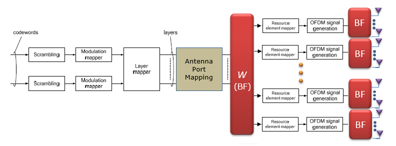
If you put these three NR diagrams next to the LTE ones from the earlier section, the visible difference is that the box labelled 'Precoding' has been replaced by a box labelled
The reason 3GPP could afford to do this is the point about antenna ports that was made earlier on this page. Because the DM-RS travels through exactly the same beam as the data it belongs to, the UE only ever sees the
This is also the practical reason why beam management in NR is described in terms of
A more detailed illustration of Hybrid Beamforming presented in this paper ([4]) is shown below. (NOTE : In real implementation, UE side antenna is not as complicated as below. In general, UE is using a few modules (panel) of antenna which is made up of several (usually 4) antenna elements. For Antenna and Beamforming on UE side, refer to this note)

This diagram is dense, but it repays a careful look, because it shows all four beamforming stages of a real mmWave link in a single picture.
- On the gNB side (left),
W is the digital precoding matrix, applied across a small number ofTXRUs (transceiver units). Each TXRU then fans out through a bank ofphase shifters , and that bank is the analog matrixP , which drives one antenna panel. This is the hybrid structure in physical form : few digital chains, many analog elements. - The X shapes drawn inside each panel are the antenna elements themselves. The two crossed lines represent the two polarizations - this is the cross polarized (+45 / -45 degree) element that is used in practically every commercial array, and it is the very same polarization pair that the φ_n co-phasing term was dealing with back in the LTE codebook.
- On the UE side (right) the structure is a mirror image : an analog receive beamforming matrix
Q in the phase shifters, and a digital combining matrixF after the TXRUs. This is the part that is easy to forget - at mmWave,the UE beamforms as well . A phone at 28 GHz carries several small panels and steers its own receive beam, which is why a beam pair (one beam at each end) rather than a single beam is what actually has to be maintained. - In the middle, the beam coming out of one gNB panel is drawn reaching the UE by bouncing off a
reflector . This is not decoration. At mmWave a reflected path is very often the only path available, which is the whole reason the beam failure recovery procedure exists in NR.
The system model written in the middle of the figure,
It is also worth noticing what this expression implies about the
YouTube
Following videos are mostly about the general concept and application of beam forming and they are not specifically limited to LTE beamforming.
- BeamForming (Feb 2011)
- 802.11ac: Why Beamforming? (May 2013)
- Antenna parameters (Feb 2013)
- Various forms of Antenna array (Feb 2013)
- Antenna array part-I (May 2013)
- Addressing LTE-A Beamforming Test Challenges: Part 1. Measurement Challenges (Oct 2016)
- Addressing LTE-A Beamforming Test Challenges: Part 2. Key Measurements (Oct 2016)
- Addressing LTE-A Beamforming Test Challenges: Part 3. Using a Multi-Channel Reference Solution (Oct 2016)
- Full-Stack Hybrid Beamforming in mmWave 5G Networks (Jun 2021)
References
These are not my posting, but I would like to recommend these for further understanding and giving you different perspective.
- [1] Digital BeamForming
- [2] TD-LTE 8-antenna dual-stream beamforming technology
- [3] Advanced antenna systems for 5G networks
- [4] Beam Management in Millimeter-Wave Communications for 5G and Beyond
YouTube - Hands on / DIY Phased Array
The videos in this second list are of a different kind from the ones above. They are not about the theory or about the 3GPP specification, but about actually building and measuring a small phased array with low cost SDR hardware. If you are the kind of person who only really believes something after seeing it work on a bench, start here.
- Build Your Own Phased Array Beamformer - Jon Kraft (2022)
- Monopulse Tracking with a Low Cost Pluto SDR - Jon Kraft (2022)
- Implementing Time Delay For a Low Cost Digital Beamformer - Jon Kraft (2022)
- Rapid Phased Array prototyping with Analog Devices and X-Microwave - Jon Kraft (2022)