Python | ShareTechnote

Panda - Basic Tutorial

In this page, I will give you some of the basic operations for Panda. I will not go very deep into Panda functions in this page. This page is just for you to try some basic things without getting scared of too complicated operation right after you installed panda package.

Pandas provides two main data structures:

DataFrame: A two-dimensional, size-mutable, and heterogeneous tabular data structure with labeled axes (rows and columns). It is similar to a SQL table or an Excel spreadsheet and is the most widely-used data structure in Pandas. DataFrames can store data of different types (e.g., integers, floats, strings, etc.) and provide a variety of functionality for handling missing data, reshaping data, merging data, and performing various data manipulation operations.
Series: A one-dimensional labeled array capable of holding any data type (integers, floats, strings, Python objects, etc.). It is similar to a column in a DataFrame, and you can think of a DataFrame as a collection of Series objects. Series provides many of the same methods and operations as DataFrames but for one-dimensional data.

Some of the key features and functionality provided by the Pandas library include:

Data I/O: Pandas can read and write data from various file formats such as CSV, Excel, JSON, SQL, and more, making it convenient for working with data from different sources.
Data Cleaning and Preprocessing: Pandas provides functionality for handling missing data, duplicates, and data type conversions. It also allows for easy renaming and reordering of columns, as well as filtering and sorting of data.
Data Transformation: Pandas allows you to reshape, pivot, and transpose data, as well as perform operations like concatenation, merging, and joining of DataFrames.
Data Aggregation and Grouping: Pandas provides the groupby functionality, allowing you to group data based on specific conditions and apply aggregation functions such as sum, average, count, or custom functions.
Time Series Analysis: Pandas has robust support for working with time series data, including handling date and time data types, resampling, time zone conversions, and more.
Data Analysis: Pandas supports descriptive statistics, correlation analysis, and other statistical functions that can help you understand and explore your data.
Data Visualization: Although Pandas is not primarily a visualization library, it provides some built-in plotting functionality that is built on top of Matplotlib, making it convenient to visualize data directly from DataFrames and Series.

The data for this tutorial is from https://support.spatialkey.com/spatialkey-sample-csv-data/ (If this link does not work, try this).

Download the file, unzip it and put it into the folder where Python is installed. Of course, you can put the file into other places. However, if you want to run the command in this tutorial as it is without modifying the data path, put the csv file in your Python installation folder.

The data structure of the csv file is as shown below.

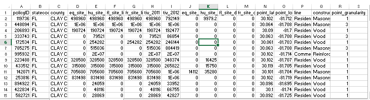
NOTE : In most case in this note, I used the table shown above, but in some examples I used another table that I used in 'Data Analysis' page.

Following is the list of basic steps that you may would go through most commonly.

Saving/Exporting to a CSV file

Importing Packages

In this tutorial, multiple packages listed below will be used. You can import all of the these package at the start or you can import them in the middle as you need it.

>>> import pandas as pd

>>> import numpy as np

>>> import matplotlib.pyplot as plt

>>> import random as rd

Read csv file

First, read the whole csv file and store the data into a variable. There are many options for read_csv() function so that you can restructure the data or read only a subset of the data. But I used the simplest way to use this function in this tutorial.

NOTE : it is assumed that you put the following csv file in c:\tmp folder.

Read as it is

Following is to read the file in the form as it is. This is the default setting.

>>> df = pd.read_csv('C:\\tmp\\FL_insurance_sample.csv')

Read without specifying row names (row index)

When read_csv() function reads csv file, it makes some guess about the column header and row number. Usually it assumes that the first row as a the column header (column title) and the first column as the row number. According to my experience, if the first column is numeric data read_csv() seems to assume that the first column is row number (not the data). Sometimes this cause problem when the first column is a part of data (not the row number). In this case, you can tell read_csv() function that this files does not have any row number as follows.

>>> df = pd.read_csv('C:\\tmp\\FL_insurance_sample.csv', index_col=False)

Read with the first n lines skipped

You can also skip the first N lines when you are reading the csv file. You would see some of the csv files which has just description of the data, not the data itself. It is usefull to understand the nature of the data, but you don't need it when it comes to real data processing.

I have a csv file that looks as follows when you read it as it is.

>>> df = pd.read_csv('Sacramentorealestatetransactions.csv')

>>> df.head()

street city zip ... price latitude longitude

0 3526 HIGH ST SACRAMENTO 95838 ... 59222 38.631913 -121.434879

1 51 OMAHA CT SACRAMENTO 95823 ... 68212 38.478902 -121.431028

2 2796 BRANCH ST SACRAMENTO 95815 ... 68880 38.618305 -121.443839

3 2805 JANETTE WAY SACRAMENTO 95815 ... 69307 38.616835 -121.439146

4 6001 MCMAHON DR SACRAMENTO 95824 ... 81900 38.519470 -121.435768

[5 rows x 12 columns]

Now I want to skip the first 2 lines (just for easy comparison) when I read the file. You can do it as shown below.

>>> df = pd.read_csv('Sacramentorealestatetransactions.csv',skiprows=2)

>>> df.head()

51 OMAHA CT SACRAMENTO 95823 ... 68212 38.478902 -121.431028

0 2796 BRANCH ST SACRAMENTO 95815 ... 68880 38.618305 -121.443839

1 2805 JANETTE WAY SACRAMENTO 95815 ... 69307 38.616835 -121.439146

2 6001 MCMAHON DR SACRAMENTO 95824 ... 81900 38.519470 -121.435768

3 5828 PEPPERMILL CT SACRAMENTO 95841 ... 89921 38.662595 -121.327813

4 6048 OGDEN NASH WAY SACRAMENTO 95842 ... 90895 38.681659 -121.351705

[5 rows x 12 columns]

Getting table dimensions (number of rows, number of colums)

Let's assume I have a table as shown below and I want to know the dimensions of the table, number of rows and number of columns.

If you just print out the table in compact form, you would get the demention at the end of the print.

>>> df

street city zip ... price latitude longitude

0 3526 HIGH ST SACRAMENTO 95838 ... 59222 38.631913 -121.434879

1 51 OMAHA CT SACRAMENTO 95823 ... 68212 38.478902 -121.431028

2 2796 BRANCH ST SACRAMENTO 95815 ... 68880 38.618305 -121.443839

3 2805 JANETTE WAY SACRAMENTO 95815 ... 69307 38.616835 -121.439146

4 6001 MCMAHON DR SACRAMENTO 95824 ... 81900 38.519470 -121.435768

.. ... ... ... ... ... ... ...

980 9169 GARLINGTON CT SACRAMENTO 95829 ... 232425 38.457679 -121.359620

981 6932 RUSKUT WAY SACRAMENTO 95823 ... 234000 38.499893 -121.458890

982 7933 DAFFODIL WAY CITRUS HEIGHTS 95610 ... 235000 38.708824 -121.256803

983 8304 RED FOX WAY ELK GROVE 95758 ... 235301 38.417000 -121.397424

984 3882 YELLOWSTONE LN EL DORADO HILLS 95762 ... 235738 38.655245 -121.075915

[985 rows x 12 columns]

You can explicitely get the number of rows and the number of columns in following ways.

>>> len(df)

985

>>> len(df.columns)

Getting the first n rows

Just for quick check after you read the csv file, you may like to print the first few rows from the file and see the overall table structure. You can easily to this with the function head() as follows.

If you call head() with default configuration, it prints out the first 5 rows of the table.

>>> df.head()

street city zip ... price latitude longitude

0 3526 HIGH ST SACRAMENTO 95838 ... 59222 38.631913 -121.434879

1 51 OMAHA CT SACRAMENTO 95823 ... 68212 38.478902 -121.431028

2 2796 BRANCH ST SACRAMENTO 95815 ... 68880 38.618305 -121.443839

3 2805 JANETTE WAY SACRAMENTO 95815 ... 69307 38.616835 -121.439146

4 6001 MCMAHON DR SACRAMENTO 95824 ... 81900 38.519470 -121.435768

[5 rows x 12 columns]

If you want to print out the header name only, you can do it by setting the number of rows in head() function.

>>> df.head(0)

Empty DataFrame

Columns: [street, city, zip, state, beds, baths, sq__ft, type, sale_date, price, latitude, longitude]

Index: []

You can print out arbitray number of rows by specifying the row numbers in head() function.

>>> df.head(3)

street city zip ... price latitude longitude

0 3526 HIGH ST SACRAMENTO 95838 ... 59222 38.631913 -121.434879

1 51 OMAHA CT SACRAMENTO 95823 ... 68212 38.478902 -121.431028

2 2796 BRANCH ST SACRAMENTO 95815 ... 68880 38.618305 -121.443839

[3 rows x 12 columns]

Adding Column Header

If the data that you read from a csv files does not have column title(header), you can add the column headers as shown the example below.

>>> df = pd.read_csv('Sacramentorealestatetransactions.csv',skiprows=2)

>>> df.head()

51 OMAHA CT SACRAMENTO 95823 ... 68212 38.478902 -121.431028

0 2796 BRANCH ST SACRAMENTO 95815 ... 68880 38.618305 -121.443839

1 2805 JANETTE WAY SACRAMENTO 95815 ... 69307 38.616835 -121.439146

2 6001 MCMAHON DR SACRAMENTO 95824 ... 81900 38.519470 -121.435768

3 5828 PEPPERMILL CT SACRAMENTO 95841 ... 89921 38.662595 -121.327813

4 6048 OGDEN NASH WAY SACRAMENTO 95842 ... 90895 38.681659 -121.351705

[5 rows x 12 columns]

Now I want to add the colum names that I defined (Actually I just copied the column name from the orignal csv file -:)

>>> cols = ['street', 'city', 'zip', 'state', 'beds', 'baths', 'sq__ft', 'type', 'sale_date', 'price', 'latitude', 'longitude'];

>>> df.columns = cols;

>>> df.head()

street city zip ... price latitude longitude

0 2796 BRANCH ST SACRAMENTO 95815 ... 68880 38.618305 -121.443839

1 2805 JANETTE WAY SACRAMENTO 95815 ... 69307 38.616835 -121.439146

2 6001 MCMAHON DR SACRAMENTO 95824 ... 81900 38.519470 -121.435768

3 5828 PEPPERMILL CT SACRAMENTO 95841 ... 89921 38.662595 -121.327813

4 6048 OGDEN NASH WAY SACRAMENTO 95842 ... 90895 38.681659 -121.351705

[5 rows x 12 columns]

Controlling the number of columns and rows for print

If you print the data table in panda, usually it prints in a compact form as shown below

>>> df.head()

street city zip ... price latitude longitude

0 3526 HIGH ST SACRAMENTO 95838 ... 59222 38.631913 -121.434879

1 51 OMAHA CT SACRAMENTO 95823 ... 68212 38.478902 -121.431028

2 2796 BRANCH ST SACRAMENTO 95815 ... 68880 38.618305 -121.443839

3 2805 JANETTE WAY SACRAMENTO 95815 ... 69307 38.616835 -121.439146

4 6001 MCMAHON DR SACRAMENTO 95824 ... 81900 38.519470 -121.435768

[5 rows x 12 columns]

You see some of the columns are hidden for simplicity. But in some case, you may want to get all the columns / rows printed out. For example, if you want to get all the columns printed out, you can change the panda option as follows.

>>> pd.set_option('display.max_columns', None)

Now print the table and it prints as follows.

>>> df.head()

street city zip state beds baths sq__ft \

0 3526 HIGH ST SACRAMENTO 95838 CA 2 1 836

1 51 OMAHA CT SACRAMENTO 95823 CA 3 1 1167

2 2796 BRANCH ST SACRAMENTO 95815 CA 2 1 796

3 2805 JANETTE WAY SACRAMENTO 95815 CA 2 1 852

4 6001 MCMAHON DR SACRAMENTO 95824 CA 2 1 797

type sale_date price latitude longitude

0 Residential Wed May 21 00:00:00 EDT 2008 59222 38.631913 -121.434879

1 Residential Wed May 21 00:00:00 EDT 2008 68212 38.478902 -121.431028

2 Residential Wed May 21 00:00:00 EDT 2008 68880 38.618305 -121.443839

3 Residential Wed May 21 00:00:00 EDT 2008 69307 38.616835 -121.439146

4 Residential Wed May 21 00:00:00 EDT 2008 81900 38.519470 -121.435768

If you want to go back to the compact print form, you can change it back as shown below.

>>> pd.set_option('display.max_columns', 7)

>>> df.head()

street city zip ... price latitude longitude

0 3526 HIGH ST SACRAMENTO 95838 ... 59222 38.631913 -121.434879

1 51 OMAHA CT SACRAMENTO 95823 ... 68212 38.478902 -121.431028

2 2796 BRANCH ST SACRAMENTO 95815 ... 68880 38.618305 -121.443839

3 2805 JANETTE WAY SACRAMENTO 95815 ... 69307 38.616835 -121.439146

4 6001 MCMAHON DR SACRAMENTO 95824 ... 81900 38.519470 -121.435768

[5 rows x 12 columns]

Extract Row with Index

Now let's take a specific row from the read csv file. For example, I want to take out the first row of the data (table) using the command as shown below.

>>> df.ix[0] // NOTE : ix[] is deprecated in latest release. you can use the following command instead.

>>> df.iloc[0]

policyID 119736

statecode FL

county CLAY COUNTY

eq_site_limit 498960

hu_site_limit 498960

fl_site_limit 498960

fr_site_limit 498960

tiv_2011 498960

tiv_2012 792149

eq_site_deductible 0

hu_site_deductible 9979.2

fl_site_deductible 0

fr_site_deductible 0

point_latitude 30.1023

point_longitude -81.7118

line Residential

construction Masonry

point_granularity 1

Name: 0, dtype: object

You can extract the multiple consecutive rows from the data (table) as shown below.

>>> df.ix[3:5] // NOTE : ix[] is deprecated in latest release. you can use the following command instead.

>>> df.iloc[3:6]

policyID statecode county eq_site_limit hu_site_limit \

3 333743 FL CLAY COUNTY 0.0 79520.76

4 172534 FL CLAY COUNTY 0.0 254281.50

5 785275 FL CLAY COUNTY 0.0 515035.62

fl_site_limit fr_site_limit tiv_2011 tiv_2012 eq_site_deductible \

3 0.0 0.0 79520.76 86854.48 0.0

4 0.0 254281.5 254281.50 246144.49 0.0

5 0.0 0.0 515035.62 884419.17 0.0

hu_site_deductible fl_site_deductible fr_site_deductible point_latitude

3 0.0 0.0 0 30.063236

4 0.0 0.0 0 30.060614

5 0.0 0.0 0 30.063236

point_longitude line construction point_granularity

3 -81.707703 Residential Wood 3

4 -81.702675 Residential Wood 1

5 -81.707703 Residential Masonry 3

You can extract multiple / non-consecutive rows using a array as shown below.

>>> df.ix[[3,5,9]] // NOTE : ix[] is deprecated in latest release. You can use the following command instead

>>> df.iloc[[3,5,9]]

policyID statecode county eq_site_limit hu_site_limit \

3 333743 FL CLAY COUNTY 0.0 79520.76

5 785275 FL CLAY COUNTY 0.0 515035.62

9 142071 FL CLAY COUNTY 705600.0 705600.00

fl_site_limit fr_site_limit tiv_2011 tiv_2012 eq_site_deductible \

3 0.0 0.0 79520.76 86854.48 0.0

5 0.0 0.0 515035.62 884419.17 0.0

9 705600.0 705600.0 705600.00 1010842.56 14112.0

hu_site_deductible fl_site_deductible fr_site_deductible point_latitude \

3 0.0 0.0 0 30.063236

5 0.0 0.0 0 30.063236

9 35280.0 0.0 0 30.100628

point_longitude line construction point_granularity

3 -81.707703 Residential Wood 3

5 -81.707703 Residential Masonry 3

9 -81.703751 Residential Masonry 1

You can get the exactly same result as above using the following command.

>>> r = [3,5,9]

>>> df.ix[r] // NOTE : ix[] is deprecated in latest release. you can use the following command instead

>>> df.iloc[r]

Extract Column with Column Name

You can extract a certain column from the csv file using the column title as shown below.

>>> df_eq = df['eq_site_limit']

You can print out the extracted data using print(). Don't worry even if the number of the extracted data is too big. I noticed that the print() print only a subset of the data as shown below.

>>> print(df_eq)

0 498960.0

1 1322376.3

2 190724.4

3 0.0

4 0.0

5 0.0

6 0.0

7 328500.0

8 315000.0

9 705600.0

10 831498.3

11 0.0

12 0.0

13 0.0

14 0.0

15 0.0

16 0.0

...

36621 0.0

36622 0.0

36623 0.0

36624 0.0

36625 0.0

36626 0.0

36627 0.0

36628 0.0

36629 0.0

36630 1297057.5

36631 173286.9

36632 1499781.6

36633 373488.3

Name: eq_site_limit, dtype: float64

You can extract the multiple columns as using the array (list) of column titles as shown below.

>>> df_eq = df[['eq_site_limit','eq_site_deductible']]

>>> print(df_eq)

eq_site_limit eq_site_deductible

0 498960.0 0.0

1 1322376.3 0.0

2 190724.4 0.0

3 0.0 0.0

4 0.0 0.0

5 0.0 0.0

6 0.0 0.0

7 328500.0 0.0

8 315000.0 0.0

9 705600.0 14112.0

10 831498.3 0.0

... ... ...

36626 0.0 0.0

36627 0.0 0.0

36628 0.0 0.0

36629 0.0 0.0

36630 1297057.5 0.0

36631 173286.9 0.0

36632 1499781.6 0.0

36633 373488.3 0.0

[36634 rows x 2 columns]

Extract Columns with Index

In this example, I will use the following table (see this note on where to get this table).

>>> df.head()

street city zip ... price latitude longitude

0 3526 HIGH ST SACRAMENTO 95838 ... 59222 38.631913 -121.434879

1 51 OMAHA CT SACRAMENTO 95823 ... 68212 38.478902 -121.431028

2 2796 BRANCH ST SACRAMENTO 95815 ... 68880 38.618305 -121.443839

3 2805 JANETTE WAY SACRAMENTO 95815 ... 69307 38.616835 -121.439146

4 6001 MCMAHON DR SACRAMENTO 95824 ... 81900 38.519470 -121.435768

[5 rows x 12 columns]

I want to get the first column of the table. you can do it as follows.

>>> df.iloc[:,0]

0 3526 HIGH ST

1 51 OMAHA CT

2 2796 BRANCH ST

3 2805 JANETTE WAY

4 6001 MCMAHON DR

...

980 9169 GARLINGTON CT

981 6932 RUSKUT WAY

982 7933 DAFFODIL WAY

983 8304 RED FOX WAY

984 3882 YELLOWSTONE LN

Name: street, Length: 985, dtype: object

You can get the multiple columns as shown below.

>>> df.iloc[:,[0,3,8]]

street state sale_date

0 3526 HIGH ST CA Wed May 21 00:00:00 EDT 2008

1 51 OMAHA CT CA Wed May 21 00:00:00 EDT 2008

2 2796 BRANCH ST CA Wed May 21 00:00:00 EDT 2008

3 2805 JANETTE WAY CA Wed May 21 00:00:00 EDT 2008

4 6001 MCMAHON DR CA Wed May 21 00:00:00 EDT 2008

.. ... ... ...

980 9169 GARLINGTON CT CA Thu May 15 00:00:00 EDT 2008

981 6932 RUSKUT WAY CA Thu May 15 00:00:00 EDT 2008

982 7933 DAFFODIL WAY CA Thu May 15 00:00:00 EDT 2008

983 8304 RED FOX WAY CA Thu May 15 00:00:00 EDT 2008

984 3882 YELLOWSTONE LN CA Thu May 15 00:00:00 EDT 2008

[985 rows x 3 columns]

Listing All the Column Names

Let's assume that I have a table as shown below.

>>> df.head()

street city zip ... price latitude longitude

0 3526 HIGH ST SACRAMENTO 95838 ... 59222 38.631913 -121.434879

1 51 OMAHA CT SACRAMENTO 95823 ... 68212 38.478902 -121.431028

2 2796 BRANCH ST SACRAMENTO 95815 ... 68880 38.618305 -121.443839

3 2805 JANETTE WAY SACRAMENTO 95815 ... 69307 38.616835 -121.439146

4 6001 MCMAHON DR SACRAMENTO 95824 ... 81900 38.519470 -121.435768

You see only some of the columns are printed and others are hidden. If you want to print out every column, see here. But in some case, you just want to know of the names of every column (not the whole dataset). In this case, you can get all the column names as shown below. There are many other ways to do the same thing, but I think these are the simplest ways.

>>> list(df.columns)

['street', 'city', 'zip', 'state', 'beds', 'baths', 'sq__ft', 'type', 'sale_date', 'price', 'latitude', 'longitude']

>>> df.columns

Index(['street', 'city', 'zip', 'state', 'beds', 'baths', 'sq__ft', 'type',

'sale_date', 'price', 'latitude', 'longitude'],

dtype='object')

Finding Column Index from Column Name

Let's assume that I have a table as shown below and I want to know of the column index for 'price' column.

>>> df.head()

street city zip ... price latitude longitude

0 3526 HIGH ST SACRAMENTO 95838 ... 59222 38.631913 -121.434879

1 51 OMAHA CT SACRAMENTO 95823 ... 68212 38.478902 -121.431028

2 2796 BRANCH ST SACRAMENTO 95815 ... 68880 38.618305 -121.443839

3 2805 JANETTE WAY SACRAMENTO 95815 ... 69307 38.616835 -121.439146

4 6001 MCMAHON DR SACRAMENTO 95824 ... 81900 38.519470 -121.435768

You can get the column index of the 'price' column using get_loc() function as shown below.

>>> df.columns.get_loc('price')

Resetting the row index

>>> df.reset_index()

>>> df.reset_index(drop = True) # This prevent the old index from being added as a data column

Extracting a Subset (Sub Table)

Using the combination of Row Extraction and Column Extraction functionalities, you can cut out a subset (a subtable) from the csv file as shown in the following examples.

>>> df_subset = df.ix[3:10][['eq_site_limit','eq_site_deductible']]

// NOTE : ix[] is deprecated in latest release. You can use the following command instead

>>> df_subset = df.loc[3:11, ['eq_site_limit','eq_site_deductible']]

// NOTE : I used loc[] instead of iloc[]. iloc[] allows only numeric data. it does not take column name.

>>> print(df_subset)

eq_site_limit eq_site_deductible

3 0.0 0.0

4 0.0 0.0

5 0.0 0.0

6 0.0 0.0

7 328500.0 0.0

8 315000.0 0.0

9 705600.0 14112.0

10 831498.3 0.0

>>> df_subset = df.ix[[3,5,10],['eq_site_limit','eq_site_deductible']]

// NOTE : ix[] is deprecated in latest release. You can use the following command instead

>>> df_subset = df.loc[[3,5,10], ['eq_site_limit','eq_site_deductible']]

// NOTE : I used loc[] instead of iloc[]. iloc[] allows only numeric data. it does not take column name.

>>> print(df_subset)

eq_site_limit eq_site_deductible

3 0.0 0.0

5 0.0 0.0

10 831498.3 0.0

If you use a random array as row index array as shown below, you can get random sampling of the csv file.

>>> rndRow = [rd.randint(0,100) for i in range(10)]

>>> df_subset = df.ix[rndRow][['eq_site_limit','eq_site_deductible']]

// NOTE : ix[] is deprecated in latest release. You can use the following command instead

>>> df_subset = df.loc[rndRow, ['eq_site_limit','eq_site_deductible']]

// NOTE : I used loc[] instead of iloc[]. iloc[] allows only numeric data. it does not take column name.

>>> print(df_subset)

eq_site_limit eq_site_deductible

34 0.0 0.0

43 213876.0 0.0

1 1322376.3 0.0

52 0.0 0.0

3 0.0 0.0

83 42300.0 0.0

15 0.0 0.0

86 0.0 0.0

11 0.0 0.0

21 0.0 0.0

Inserting a Column

Let's assume that I have a table as shown below and I want to change the price in other currency with the application of a specific exchange rate and add the result as a new column.

>>> header = df.head()

>>> print(header)

street city zip ... price latitude longitude

0 3526 HIGH ST SACRAMENTO 95838 ... 59222 38.631913 -121.434879

1 51 OMAHA CT SACRAMENTO 95823 ... 68212 38.478902 -121.431028

2 2796 BRANCH ST SACRAMENTO 95815 ... 68880 38.618305 -121.443839

3 2805 JANETTE WAY SACRAMENTO 95815 ... 69307 38.616835 -121.439146

4 6001 MCMAHON DR SACRAMENTO 95824 ... 81900 38.519470 -121.435768

now I want to extract the 'price' column, apply with an exchange rate and save it into a new dataset.

>>> df_price_cad = df['price'] * 1.4

>>> print(df_price_cad)

0 82910.8

1 95496.8

2 96432.0

3 97029.8

4 114660.0

...

980 325395.0

981 327600.0

982 329000.0

983 329421.4

984 330033.2

Name: price, Length: 985, dtype: float64

Now I want to add this dataset as a new column right next to the 'price' column. This mean 'Insert the data df_price_cad at the column index 10 of the data set df with the column title = 'price_CAD'. (NOTE : how can I know that the column index right next to 'price' column is 10 ? See Finding the column index from the column name if you want to know the details).

>>> df.insert(10, 'price_CAD', df_price_cad)

>>> df.head()

street city zip ... price_CAD latitude longitude

0 3526 HIGH ST SACRAMENTO 95838 ... 82910.8 38.631913 -121.434879

1 51 OMAHA CT SACRAMENTO 95823 ... 95496.8 38.478902 -121.431028

2 2796 BRANCH ST SACRAMENTO 95815 ... 96432.0 38.618305 -121.443839

3 2805 JANETTE WAY SACRAMENTO 95815 ... 97029.8 38.616835 -121.439146

4 6001 MCMAHON DR SACRAMENTO 95824 ... 114660.0 38.519470 -121.435768

[5 rows x 13 columns]

Deleting Columns

Let's assume that I have a table as shown below and I want to delete the colum 'zip'.

>>> header = df.head()

>>> print(header)

street city zip ... price latitude longitude

0 3526 HIGH ST SACRAMENTO 95838 ... 59222 38.631913 -121.434879

1 51 OMAHA CT SACRAMENTO 95823 ... 68212 38.478902 -121.431028

2 2796 BRANCH ST SACRAMENTO 95815 ... 68880 38.618305 -121.443839

3 2805 JANETTE WAY SACRAMENTO 95815 ... 69307 38.616835 -121.439146

4 6001 MCMAHON DR SACRAMENTO 95824 ... 81900 38.519470 -121.435768

>>> del df['zip']

>>> df.head()

street city state ... price_CAD latitude longitude

0 3526 HIGH ST SACRAMENTO CA ... 82910.8 38.631913 -121.434879

1 51 OMAHA CT SACRAMENTO CA ... 95496.8 38.478902 -121.431028

2 2796 BRANCH ST SACRAMENTO CA ... 96432.0 38.618305 -121.443839

3 2805 JANETTE WAY SACRAMENTO CA ... 97029.8 38.616835 -121.439146

4 6001 MCMAHON DR SACRAMENTO CA ... 114660.0 38.519470 -121.435768

[5 rows x 12 columns]

You can do the same thing as follows. With drop() function, you can delete column or row by specifying 0 or 1 at the second argument. '1' in the second argument mean 'column', 0 mean row.

>>> df = df.drop('zip',1)

You may notice in the above example, we needed to reassign the df.drop() result to the variable. If you want to get the deleted result without the reassignment, you can do it as shown below.

>>> df.drop('zip', axis=1, inplace=True)

If you want to delete the multiple columns at once, you can do it as follows.

>>> df.drop(['city', 'zip'], axis=1, inplace=True)

If you want to delete the columns using the index number rather than column names, you can do it as follows.

>>> df.drop(df.columns[[1,2,5]], axis=1, inplace=True)

Processing a Column data with Map()

Let's suppose I have a column data as below and I want to split this data into separate items (like date, month, time, year etc).

>>> saledate = df['sale_date']

>>> saledate.head()

0 Wed May 21 00:00:00 EDT 2008

1 Wed May 21 00:00:00 EDT 2008

2 Wed May 21 00:00:00 EDT 2008

3 Wed May 21 00:00:00 EDT 2008

4 Wed May 21 00:00:00 EDT 2008

Name: sale_date, dtype: object

Map with lambda function (inline function)

One simple way to do this is to use Map() funtion as shown below (If you are not faimilar with map(), see this note first).

>>> saledate_item = saledate.map(lambda x:x.split(" "))

>>> saledate_item.head()

0 [Wed, May, 21, 00:00:00, EDT, 2008]

1 [Wed, May, 21, 00:00:00, EDT, 2008]

2 [Wed, May, 21, 00:00:00, EDT, 2008]

3 [Wed, May, 21, 00:00:00, EDT, 2008]

4 [Wed, May, 21, 00:00:00, EDT, 2008]

Name: sale_date, dtype: object

Map with a pre-defined function

lamda function is simple and handy, but it would be a little bit trick to do anything complicated. In this case, you can define the procedure as a predefined function and apply it in map() function as shown in the following example.

def mm_yyyy(d) :

dList = d.split(" ");

dStr = dList[1] + ":" + dList[5];

return dStr;

>>> df_mm_yyyy = df['sale_date'].map(mm_yyyy);

>>> df_mm_yyyy

0 May:2008

1 May:2008

2 May:2008

3 May:2008

4 May:2008

...

980 May:2008

981 May:2008

982 May:2008

983 May:2008

984 May:2008

Name: sale_date, Length: 985, dtype: object

Save/Export a Dataset to CSV file

You can save/export a data set that you created to a csv file using to_csv() function as shown in the examples shown in this section.

>>> df_subset = df.loc[[3,5,9],['street','city']]

>>> print(df_subset)

street city

3 2805 JANETTE WAY SACRAMENTO

5 5828 PEPPERMILL CT SACRAMENTO

9 7325 10TH ST RIO LINDA

Save it as it is

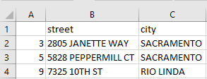
If you save the data set to csv file in default configuration, it saves not only the data but also the index and the column name as shown below.

>>> df_subset.to_csv('C:\\tmp\\df_subset.csv')

Save it without row index (Supressing the row index)

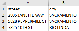
If you don't want to save the index value, you can suppress it as follows.

>>> df_subset.to_csv('C:\\tmp\\df_subset.csv',index=False)

Save it without Column Header

If you don't want to save the header (column name), you can suppress it as follows.

>>> df_subset.to_csv('C:\\tmp\\df_subset.csv',header=False)

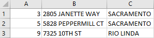
Save it without Row index and Column Header

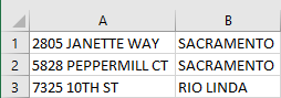
If you don't want to suppress both index and header, you can do it as follows.

>>> df_subset.to_csv('C:\\tmp\\df_subset.csv',index=False,header=False)

Save it with your own column header

If you want to save the file with your own column name, you can specify the column name as shown below.

>>> df_subset.to_csv('C:\\tmp\\df_subset.csv',header=['column1','column2'])

Chaning Numeric Type

You can change the type of numeric data as follows. Note that all the data in the dataset should be numeric data for the numeric type specification to be applied. Otherwise, you would get errors.

>>> df['longitude'].astype(int)

0 -121

1 -121

2 -121

3 -121

4 -121

...

980 -121

981 -121

982 -121

983 -121

984 -121

Name: longitude, Length: 985, dtype: int32

>>> df['longitude'].astype(float)

0 -121.434879

1 -121.431028

2 -121.443839

3 -121.439146

4 -121.435768

...

980 -121.359620

981 -121.458890

982 -121.256803

983 -121.397424

984 -121.075915

Name: longitude, Length: 985, dtype: float64

Replacing NaN with 0

In many cases, you may get a data set (usually as a result of numerical operations) with a lot of NaN but you don't like it.

>>> BedCountInCity = df.pivot_table(values='price',index=['city'],columns=['beds'],aggfunc=lambda x: x.count())

>>> BedCountInCity.head()

beds 0 1 2 ... 5 6 8

city ...

ANTELOPE NaN NaN 3.0 ... 3.0 NaN NaN

AUBURN NaN NaN 2.0 ... NaN NaN NaN

CAMERON PARK 1.0 NaN 3.0 ... NaN NaN NaN

CARMICHAEL NaN NaN 4.0 ... NaN NaN NaN

CITRUS HEIGHTS NaN NaN 4.0 ... 1.0 NaN NaN

[5 rows x 8 columns]

You can easily replace the NaN with a specific number (usually 0) as shown below.

>>> BedCountInCity.fillna(0)

beds 0 1 2 ... 5 6 8

city ...

ANTELOPE 0.0 0.0 3.0 ... 3.0 0.0 0.0

AUBURN 0.0 0.0 2.0 ... 0.0 0.0 0.0

CAMERON PARK 1.0 0.0 3.0 ... 0.0 0.0 0.0

CARMICHAEL 0.0 0.0 4.0 ... 0.0 0.0 0.0

CITRUS HEIGHTS 0.0 0.0 4.0 ... 1.0 0.0 0.0

COOL 0.0 0.0 0.0 ... 0.0 0.0 0.0

DIAMOND SPRINGS 0.0 0.0 0.0 ... 0.0 0.0 0.0

EL DORADO 0.0 0.0 1.0 ... 0.0 0.0 0.0

Converting List data to a Table (DataFormatter)

I have a list data as shown below and I want to convert this data into a pands table (dataformatter). NOTE : See this if you want to know how I got this data.

>>> df_saledate_item

sale_date

0 [Wed, May, 21, 00:00:00, EDT, 2008]

1 [Wed, May, 21, 00:00:00, EDT, 2008]

2 [Wed, May, 21, 00:00:00, EDT, 2008]

3 [Wed, May, 21, 00:00:00, EDT, 2008]

4 [Wed, May, 21, 00:00:00, EDT, 2008]

.. ...

980 [Thu, May, 15, 00:00:00, EDT, 2008]

981 [Thu, May, 15, 00:00:00, EDT, 2008]

982 [Thu, May, 15, 00:00:00, EDT, 2008]

983 [Thu, May, 15, 00:00:00, EDT, 2008]

984 [Thu, May, 15, 00:00:00, EDT, 2008]

[985 rows x 1 columns]

You can convert this list into a panda table as shown below.

>>> df_saledate_item = pd.DataFrame(saledate_item.tolist(),columns=["Day","Month","Date","Time","Zone","Year"])

>>> df_saledate_item

Day Month Date Time Zone Year

0 Wed May 21 00:00:00 EDT 2008

1 Wed May 21 00:00:00 EDT 2008

2 Wed May 21 00:00:00 EDT 2008

3 Wed May 21 00:00:00 EDT 2008

4 Wed May 21 00:00:00 EDT 2008

.. ... ... ... ... ... ...

980 Thu May 15 00:00:00 EDT 2008

981 Thu May 15 00:00:00 EDT 2008

982 Thu May 15 00:00:00 EDT 2008

983 Thu May 15 00:00:00 EDT 2008

984 Thu May 15 00:00:00 EDT 2008

[985 rows x 6 columns]

Combining Two Tables in Columns

Let's suppose I have two tables as shown below and I want to join the two tables in Column.

this is the first table named df.

>>> df.head()

street city zip ... price latitude longitude

0 3526 HIGH ST SACRAMENTO 95838 ... 59222 38.631913 -121.434879

1 51 OMAHA CT SACRAMENTO 95823 ... 68212 38.478902 -121.431028

2 2796 BRANCH ST SACRAMENTO 95815 ... 68880 38.618305 -121.443839

3 2805 JANETTE WAY SACRAMENTO 95815 ... 69307 38.616835 -121.439146

4 6001 MCMAHON DR SACRAMENTO 95824 ... 81900 38.519470 -121.435768

[5 rows x 12 columns]

Just for the reference, let's list all the column names.

>>> list(df.columns)

['street', 'city', 'zip', 'state', 'beds', 'baths', 'sq__ft', 'type', 'sale_date', 'price', 'latitude', 'longitude']

Now I have another table shown below. (NOTE : For your reference, this table is made from a sale_date in the table df. You may refer to this section if you want to know how I created this table).

>>> df_saledate_item.head()

Day Month Date Time Zone Year

0 Wed May 21 00:00:00 EDT 2008

1 Wed May 21 00:00:00 EDT 2008

2 Wed May 21 00:00:00 EDT 2008

3 Wed May 21 00:00:00 EDT 2008

4 Wed May 21 00:00:00 EDT 2008

Now I want to combine the two table df and df_saledate_item into a new table in columns.

NOTE : axis = 1 parameter is key in this case. It specify 'column', if you omit it or set it to 'axis = 0', the concat() combines the tables in row.

>>> df_new_dateformat = pd.concat([df,df_saledate_item],axis=1)

>>> df_new_dateformat.head()

street city zip state ... Date Time Zone Year

0 3526 HIGH ST SACRAMENTO 95838 CA ... 21 00:00:00 EDT 2008

1 51 OMAHA CT SACRAMENTO 95823 CA ... 21 00:00:00 EDT 2008

2 2796 BRANCH ST SACRAMENTO 95815 CA ... 21 00:00:00 EDT 2008

3 2805 JANETTE WAY SACRAMENTO 95815 CA ... 21 00:00:00 EDT 2008

4 6001 MCMAHON DR SACRAMENTO 95824 CA ... 21 00:00:00 EDT 2008

[5 rows x 18 columns]

Now print all the column names and see if the new table contains every columns from the two tables.

>>> list(df_new_dateformat.columns)

['street', 'city', 'zip', 'state', 'beds', 'baths', 'sq__ft', 'type', 'sale_date', 'price', 'latitude', 'longitude', 'Day', 'Month', 'Date', 'Time', 'Zone', 'Year']

Filter

All the examples in this section is based on a table shown below. I would not print out this original table in every example unless it is really necessary.

>>> df

street city zip ... price latitude longitude

0 3526 HIGH ST SACRAMENTO 95838 ... 59222 38.631913 -121.434879

1 51 OMAHA CT SACRAMENTO 95823 ... 68212 38.478902 -121.431028

2 2796 BRANCH ST SACRAMENTO 95815 ... 68880 38.618305 -121.443839

3 2805 JANETTE WAY SACRAMENTO 95815 ... 69307 38.616835 -121.439146

4 6001 MCMAHON DR SACRAMENTO 95824 ... 81900 38.519470 -121.435768

.. ... ... ... ... ... ... ...

980 9169 GARLINGTON CT SACRAMENTO 95829 ... 232425 38.457679 -121.359620

981 6932 RUSKUT WAY SACRAMENTO 95823 ... 234000 38.499893 -121.458890

982 7933 DAFFODIL WAY CITRUS HEIGHTS 95610 ... 235000 38.708824 -121.256803

983 8304 RED FOX WAY ELK GROVE 95758 ... 235301 38.417000 -121.397424

984 3882 YELLOWSTONE LN EL DORADO HILLS 95762 ... 235738 38.655245 -121.075915

[985 rows x 12 columns]

The list of column names are as follows.

>>> list(df.columns)

['street', 'city', 'zip', 'state', 'beds', 'baths', 'sq__ft', 'type', 'sale_date', 'price', 'latitude', 'longitude']

Selecting Rows with a specified column value

This example shows all the rows where the city name is 'ELK GROVE'

>>> df[df['city']=='ELK GROVE']

street city ... latitude longitude

30 5201 LAGUNA OAKS DR Unit 140 ELK GROVE ... 38.423251 -121.444489

34 5201 LAGUNA OAKS DR Unit 162 ELK GROVE ... 38.423251 -121.444489

42 8718 ELK WAY ELK GROVE ... 38.416530 -121.379653

50 9417 SARA ST ELK GROVE ... 38.415518 -121.370527

66 7005 TIANT WAY ELK GROVE ... 38.422811 -121.423285

.. ... ... ... ... ...

964 10085 ATKINS DR ELK GROVE ... 38.390893 -121.437821

965 9185 CERROLINDA CIR ELK GROVE ... 38.424497 -121.426595

975 5024 CHAMBERLIN CIR ELK GROVE ... 38.389756 -121.446246

979 1909 YARNELL WAY ELK GROVE ... 38.417382 -121.484325

983 8304 RED FOX WAY ELK GROVE ... 38.417000 -121.397424

[114 rows x 12 columns]

Selecting Rows with multiple column values in OR condition

If you want to filter the rows with multiple OR criteria, you can do as show below.

If the criteria is string comparison or comparing with any of listable items, you can simply do it as shown below.

>>> df[df['city'].isin(['ELK GROVE','SACRAMENTO'])]

street city zip ... price latitude longitude

0 3526 HIGH ST SACRAMENTO 95838 ... 59222 38.631913 -121.434879

1 51 OMAHA CT SACRAMENTO 95823 ... 68212 38.478902 -121.431028

2 2796 BRANCH ST SACRAMENTO 95815 ... 68880 38.618305 -121.443839

3 2805 JANETTE WAY SACRAMENTO 95815 ... 69307 38.616835 -121.439146

4 6001 MCMAHON DR SACRAMENTO 95824 ... 81900 38.519470 -121.435768

.. ... ... ... ... ... ... ...

978 5601 REXLEIGH DR SACRAMENTO 95823 ... 230000 38.445342 -121.441504

979 1909 YARNELL WAY ELK GROVE 95758 ... 230000 38.417382 -121.484325

980 9169 GARLINGTON CT SACRAMENTO 95829 ... 232425 38.457679 -121.359620

981 6932 RUSKUT WAY SACRAMENTO 95823 ... 234000 38.499893 -121.458890

983 8304 RED FOX WAY ELK GROVE 95758 ... 235301 38.417000 -121.397424

[553 rows x 12 columns]

Or you can do it using the '|' operator as shown below.

>>> df[(df['city']=='ELK GROVE') | (df['city']=='SACRAMENTO')]

street city zip ... price latitude longitude

0 3526 HIGH ST SACRAMENTO 95838 ... 59222 38.631913 -121.434879

1 51 OMAHA CT SACRAMENTO 95823 ... 68212 38.478902 -121.431028

2 2796 BRANCH ST SACRAMENTO 95815 ... 68880 38.618305 -121.443839

3 2805 JANETTE WAY SACRAMENTO 95815 ... 69307 38.616835 -121.439146

4 6001 MCMAHON DR SACRAMENTO 95824 ... 81900 38.519470 -121.435768

.. ... ... ... ... ... ... ...

978 5601 REXLEIGH DR SACRAMENTO 95823 ... 230000 38.445342 -121.441504

979 1909 YARNELL WAY ELK GROVE 95758 ... 230000 38.417382 -121.484325

980 9169 GARLINGTON CT SACRAMENTO 95829 ... 232425 38.457679 -121.359620

981 6932 RUSKUT WAY SACRAMENTO 95823 ... 234000 38.499893 -121.458890

983 8304 RED FOX WAY ELK GROVE 95758 ... 235301 38.417000 -121.397424

[553 rows x 12 columns]

Concatenating Tables

This section will show you how to concatenate multiple tables. Depending on the structure of the table, the structure of the concatenated table would vary.

To make it easier to check the result of the concatenation, I will create simple tables as shown below rather than the one from csv files.

import pandas as pd

df1 = pd.DataFrame({'A': ['A0', 'A1', 'A2', 'A3'],

'B': ['B0', 'B1', 'B2', 'B3']});

df2 = pd.DataFrame({'A': ['A4', 'A5', 'A6', 'A7'],

'B': ['B4', 'B5', 'B6', 'B7']});

df3 = pd.DataFrame({'A': ['A8', 'A9', 'A10', 'A11'],

'C': ['C0', 'C1', 'C2', 'C3']});

df4 = pd.DataFrame({'A': ['A0', 'A1', 'A2', 'A3'],

'D': ['D0', 'C1', 'C2', 'C3']});

For visualization of structure of each table, let's print out each of table and see how it looks like.

>>> df1

A B

0 A0 B0

1 A1 B1

2 A2 B2

3 A3 B3

>>> df2

A B

0 A4 B4

1 A5 B5

2 A6 B6

3 A7 B7

>>> df3

A C

0 A8 C0

1 A9 C1

2 A10 C2

3 A11 C3

>>> df4

A D

0 A0 D0

1 A1 C1

2 A2 C2

3 A3 C3

Now let's concatenate these tables and see how the result look like.

>>> df_concat = pd.concat([df1,df2]);

>>> df_concat

A B

0 A0 B0

1 A1 B1

2 A2 B2

3 A3 B3

0 A4 B4

1 A5 B5

2 A6 B6

3 A7 B7

>>> df_concat = pd.concat([df1,df3]);

>>> df_concat

A B C

0 A0 B0 NaN

1 A1 B1 NaN

2 A2 B2 NaN

3 A3 B3 NaN

0 A8 NaN C0

1 A9 NaN C1

2 A10 NaN C2

3 A11 NaN C3

>>> df_concat = pd.concat([df1,df4]);

>>> df_concat

A B D

0 A0 B0 NaN

1 A1 B1 NaN

2 A2 B2 NaN

3 A3 B3 NaN

0 A0 NaN D0

1 A1 NaN C1

2 A2 NaN C2

3 A3 NaN C3

Converting a List to a Panda DataFrame

Let's suppose I have a list shown below and I want to convert it into a pandas table so that I can use all the handy functions to my list.

>>> myList = [[1,2,3],[4,5,6],[7,8,9]]

>>> myList

[[1, 2, 3], [4, 5, 6], [7, 8, 9]]

You can easily convert this list into a pandas table as shown below (Super simple !!!!)

>>> df = pd.DataFrame(myList)

>>> df

0 1 2

0 1 2 3

1 4 5 6

2 7 8 9

Then you can add your own column header as shown below if you like

>>> df.columns = ['item 1','item2','item3'];

>>> df

item 1 item2 item3

0 1 2 3

1 4 5 6

2 7 8 9

Plot Data

You can easily visualize (e.g, plot) the data using functions in matplotlib as shown in this section.

First, you need to import the matplotlib package as shown below.

>>> import matplotlib.pyplot as plt

# in manu tutorial, they say 'import matplotlib as plt' but this didn't work in my setup. When I tried plot() function, it gave me an errror as shown below. So I tried 'import matplotlib.pyplot as plt' and it worked.

>>> plt.plot(df_eq)

Traceback (most recent call last):

File "<stdin>", line 1, in <module>

AttributeError: module 'matplotlib' has no attribute 'plot'

Then extract a dataset as in the following example.

>>> df_eq = df['eq_site_limit']

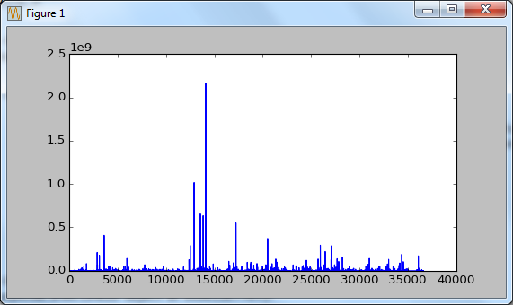
Then plot it as shown below. However, just running a plot() function would not display any graph. It just create a plot in the memory without displaying it on the screen.

>>> plt.plot(df_eq)

[<matplotlib.lines.Line2D object at 0x0612E770>]

In order to display the plot, you need to run show() function as shown below.

>>> plt.show()