In any wireless communication device, we have to go through two large group of testing. One for testing transmission path and the other for testing recieve path. That split decides more than the chapter numbering. Each path needs a different instrument and a different kind of verdict. On the transmit path the equipment listens, and what it reads out is a power, a modulation quality or a frequency error. On the receive path the equipment generates instead. The UE's own report becomes the measurement, which is why most of chapter 7 produces a throughput figure rather than a level. One warning before the rest of the page. The two paths are separate on paper but share hardware in the device. The reference sensitivity test is run with the transmitter at maximum output power, which makes the receiver figure depend on the transmitter.

• LTE RF Measurement Items
• Snapshots of LTE Uplink Signals for RF Testing
• Challenges for LTE RF Testing
• LTE Specific Measurement
• MPR - Maximum Power Reduction
• IBE - In-Band Emission
• Power Control - Absolute Power Tolerance
• Power Control - Relative Power Tolerance
• Aggregate Power Control Tolerance
• RF Test Equipment/UE Connection Diagram
• Protocol Sequence for RF Conformance Test
• RF Conformance Test - TRX Conformance - 36.521-1
• RF Conformance Test - RRM Conformance - 36.521-3
• Overview on RF/PHY Performance Test
• Test Case Description
• 36.521-1 : 6.2.2 UE Maximum Output Power
• 36.521-1 : 7.3 Reference sensitivity level
• Thinking over a cup of coffee
• Reference

For a wireless communication device to work properly, it should meet following hardware requirement

i) The device should transmit the signal which is strong enough power to make it sure it reaches the other party of the communication.

ii) The device should not transmit the signal which is so strong that it interfere the communication between other parties.

iii) The device should transmit the signal with good enough quality which can be decoded/corrected by the other party.

iv) The device should transmit the signal in the exact frequency that has been allocated for the communication.

v) The device should not generate any noise out side of the frequency area that has been allocated for the device.

If any of these condition deviate too much from the specification, the device cannot communicate with the other party or let some other device to communicate. In terms of measurement equipment, item i) and ii) belong to "power measurement", item iii) is related to "Modulation Analysis" and item iv) falls into "Frequency Error measurement". Item v) is also a kind of "power measurement", but the measurement area in frequency domain is different from item i) & item ii). Anyway if you have any equipment that can perform the following three measurement for your communication technology, you can do the most critical part of transmission path.

a) Power Measurement

b) Modulation Analysis

c) Frequency Error Measurement

Now let's think about the recieve path measurement. What would be the most important reciever characteristics for the communication device ?

i) The reciever must be able to decode successfuly the signal coming from a transmitter even though the signal strength is very low.

ii) The reciever must be able to decode successfuly the signal coming from a transmitter even when there are a certain level of noise around the signal.

In terms of measurement logic, item i) and ii) are the same. Equipment sends a pattern of the known signal and let the reciever decode it and compare the original signal from the equipment and the decoded signal by reciever and how much different they are. The more different they are, the poorer reciever quality it is. We call this method "BER(Bit Error Rate) measurement". Item i) measures BER when the input signal to the device is very low and Item ii) measures BER when there are noise to the input signal.

Before we go forward to LTE measurement, pick any technology you are already familiar with and make a list of measurement on your test plan and try to map those items with the measurement principles I described above. Once you are familiar with this mapping, you will understand LTE measurement items more easily.

LTE RF Measurement Items

Now let's look a little bit detail into LTE RF measurement. First thing I have done is to make a list of measurement items from 3GPP 36.521-1 and try to map my measurement principles with each of the measurement items.

Here goes the Transmitter measurement items first. You see a lot of "Power Measurement" and some of "Modulation Analysis". Why do we have so many different power measurement and so many different Modulation Analysis. How do they differ from each other ? This is the question you have to find answers on your own. The answer itself is described in 3GPP 36.521-1 but the question is how much I can understand what is described there just by reading it.

The first step would be to read "Test Purpose", "Initial Condition", "Test Procedure" section of each test case as often as possible and try at least to be familiar to each test case.

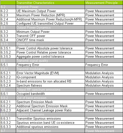
Twenty one test items in the left column, and three measurement principles in the right one. That ratio is the whole point of the table.

• The left column is 36.521-1 clause numbering : 6.2 Transmit Power, 6.3 Output Power Dynamics, 6.5 Transmit signal quality, 6.6 Output RF spectrum emissions and 6.7 Transmit Intermodulation.
• Sixteen of the rows say Power Measurement : everything under 6.2, 6.3, 6.6 and 6.7 reduces to measuring power in some band.
• Only the four rows under 6.5.2 need Modulation Analysis : EVM, IQ-component, In-band emissions for non allocated RB and Spectrum flatness.
• One row stands alone : 6.5.1 Frequency Error is the only item measured as frequency error.
• What changes between rows is the band, not the method : 6.6.1 measures occupied bandwidth and 6.6.2.3 measures the adjacent channel. Both are a power reading over a stated span.
• The grouping rows carry no principle : 6.3.5 Power Control and 6.6.2 Out of band emission are headings inside the specification, and their children carry the work.

Here goes the reciever measurement items.

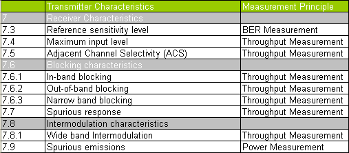
Nine receiver items, and the same collapse happens. Seven of them are one measurement with the interference moved around.

• Seven rows say Throughput Measurement : 7.4 Maximum input level, 7.5 ACS, the three blocking rows under 7.6, 7.7 Spurious response and 7.8.1 Wide band Intermodulation.
• 7.3 Reference sensitivity level is the exception : it is the only receiver row measured as BER rather than as throughput.
• 7.9 Spurious emissions is a power measurement : it sits in the receiver chapter but measures what the receiver leaks back out, so the principle is the transmitter one.
• The difference between the throughput rows is where the interference sits : in band for 7.6.1, out of band for 7.6.2 and narrow band for 7.6.3. A pair of tones does it for 7.8.1.
• The column header reads Transmitter Characteristics : that heading was carried over from the transmitter table. The group row underneath it correctly says 7 Receiver Characteristics.

• Three principles cover the transmitter and three cover the receiver : power, modulation and frequency on one side, throughput, BER and power on the other.
• Learn the principle once and the test list stops being long : thirty rows across the two tables reduce to six things a measuring instrument actually does.
• The clause number tells you which instrument you need : anything under 6.5.2 needs a demodulator. Everything else under chapter 6 needs a power meter or an analyser.
• Chapter 7 needs a signal generator more than an analyser : seven of its nine rows are about what the tester adds to the downlink, not about what the UE sends.

Snapshots of LTE Uplink Signals for RF Testing

As I mentioned earlier, it is not easy to understand all the details of LTE RF Measurement just by reading the specification. I have read the test case purpose, "Initial Condition", "Test Procedure" over and over.. but still everything is vague. As I try to get more into details, the first obstacles that blocks me is a lot of complicated tables describing the test condition. Of course we saw this kind of tables in other technology specification like CDMA, WCDMA but it seems the tables for LTE measurement looks bigger and more complicated. So I decided to see some of the signal patterns described in the specification on spectrum analyzer so that I can get some intuitive idea of the overall RF characteristics of each condition.

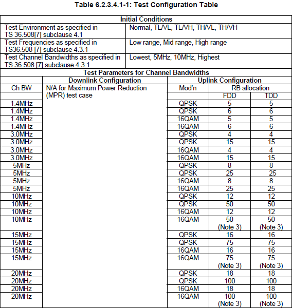
For example, following table shows the test condition for each of subtests for MPR (Maximum Power Reduction). If you see the column Uplink Configuration - RB allocation. You will see various cases of resource block allocation for the same Ch BW. Some of the sub tests uses 'Max RB number' (FULL RBs) for the specific channel BW, but some of the subtests are using the number of RBs which is smaller than the Max number of RB (Partial RBs).

Full RB Signals

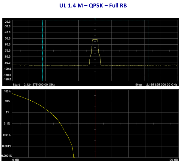
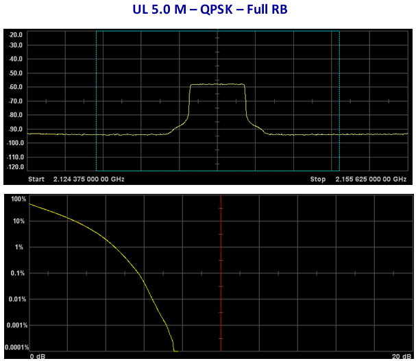
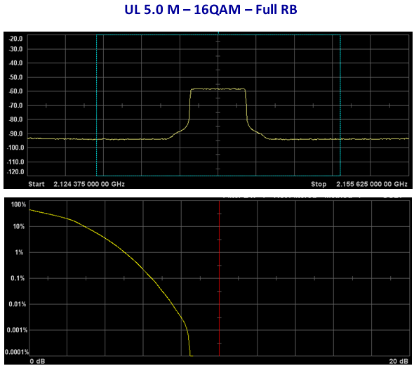
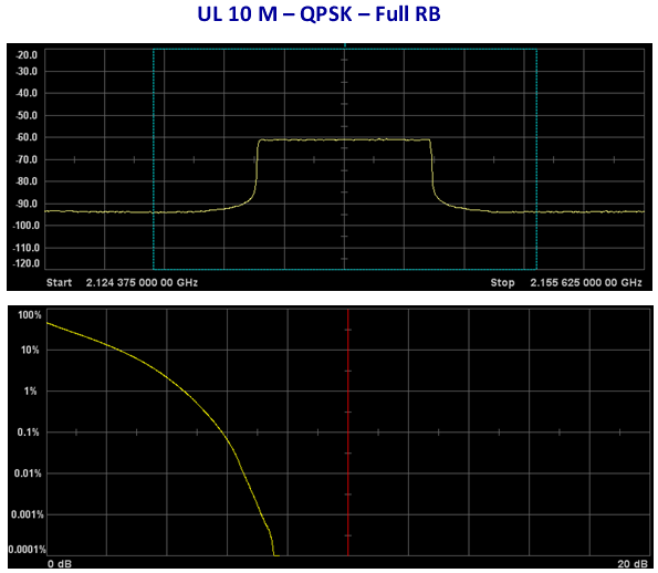
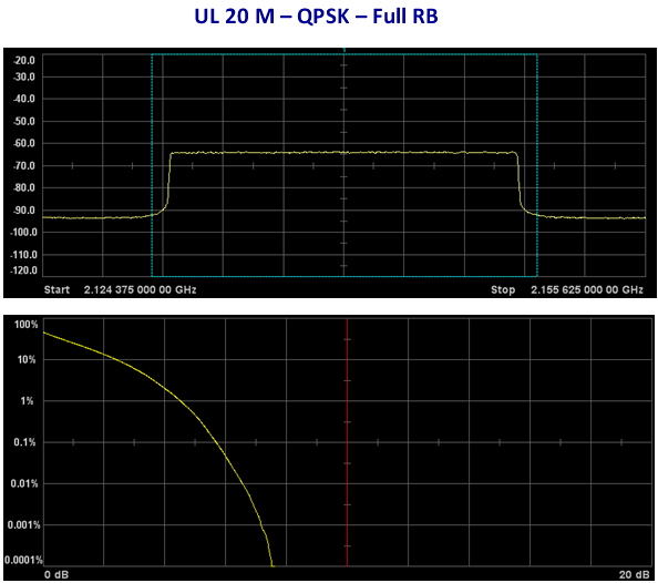
Every trace here is on the same span and the same scale. So the pictures can be compared directly rather than one at a time.

• The span never changes : every upper pane runs from 2.124 375 000 00 GHz to 2.155 625 000 00 GHz. That is 31.25 MHz, with 10 dB per vertical division.
• The occupied width tracks the channel bandwidth : the 1.4 MHz trace is a narrow bump and the 20 MHz trace almost fills the marked region.
• The flat top drops as the allocation widens : about -50 dBm at 1.4 MHz against about -65 dBm at 20 MHz. A similar total power is spread over more subcarriers.
• The noise floor stays at about -93 dBm throughout : it belongs to the instrument, not to the signal. So it is the fixed reference in every picture.
• QPSK and 16QAM look identical in the upper pane : the 5 MHz pair differs only in the lower pane, where the 16QAM curve runs further to the right.
• The lower pane is a CCDF and its axis is 0 to 20 dB : the further right the curve reaches, the higher the peak to average ratio of the waveform.

Partial RB signals

In case of allocating the number of RBs less than the max RBs (especially when the number of RB is less than 1/2 Max RBs, there can be so many different cases depending on the location of the signal. For example, the signal can be located at the left most side of the channel or at the center or at the right most side of the channel. Theoretically, it can be located in anywhere in the band, but RF conformance specifies only three locations as a test point which is Low range, Mid range, High range.  Low range means that the signal start from the left most side of the channel, Mid means the signal is located at the center of the channel, High range means the signal is at the right most side of the channel.

Following sample signals are from a vector signal generator which generate a very good quality signal and the power is also very low, so you see only the signal part without any carrier leakage or in-band image. But in reality, you will see the carrier leakage and in-band image signal in most of the case.

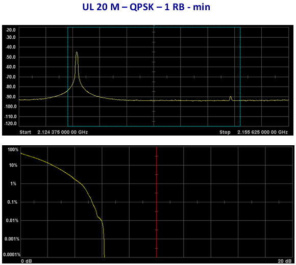
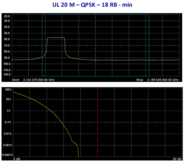
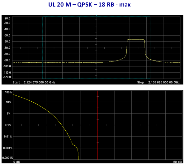
Same channel, same modulation, three allocations. What moves is where the energy sits and how peaky it is.

• One resource block is the tallest trace on the page : a single narrow spike reaching about -45 dBm, because the whole transmission is concentrated in one block.
• It also has the lowest peak to average ratio : its CCDF curve falls fastest of the three. That is what a near single carrier waveform does.
• A second small bump sits near the far marker : about -88 dBm at the opposite edge of the channel. That is the kind of product the in-band emission test is built to find.
• The 18 RB pair is the same block at opposite ends : the low placement sits against the left marker and the high placement against the right one. Both have a flat top near -62 dBm.
• The emission skirt always points inward : on the low placement it slopes to the right, on the high placement to the left. In both cases it runs across the unallocated blocks.

• Bandwidth, modulation and allocation each change a different thing : bandwidth changes the width, allocation changes the height and the position, and modulation changes only the CCDF.
• A narrow allocation is not a gentle one : one resource block gives the highest trace on the screen. So an emission limit is easiest to miss where the least is being sent.
• The unallocated part of the channel is never empty : every picture with a partial allocation shows energy where nothing was scheduled.

Even though we have new technology every couple of years and LTE is new to many people, RF test and measurement technology have a lot in common with other wireless communication technology. If you had experience with any wireless technology, eg CDMA, GSM, WCDMA, Bluetooth, WLAN, you may find the common logics in LTE.

Challenges for LTE RF Testing

One of the biggest challenges in LTE measurement for UE development or test engineer would be that there are too many sub tests with too many different parameter settings.Before I get into details, I want to briefly skim through overall RF measurement from C2K.

I don't have much experience with C2K measurement, but with only a little experience I could tell there are much fewer measurement items in this area comparing to WCDMA/HSDPA and even comparing to GSM/GPRS. As far as I remember, following is allmost all that I did for C2K.

i) Total Channel Power

ii) CDP (Code Domain Power)

iii) Rho

iv) Spectrum Emission

v) ACLR

vi) OBW (Occupied Bandwidth)

But the items listed above is more than what I experienced in C2K. For conformance, I think we may have to go through all of these items. But since C2K is very mature technology now, in the RF part developmental stage we wouldn't go through all of these items. In an extreme case that I heard of was "just measure total power, if there is no problem with it. usually no problem with other parts".

Now let's look into WCDMA. For WCDMA R99 (Non HSPA), If I briefly put the list,

i) Max Power

ii) Min Power

iii) On/Off Power

iv) RACH Power

v) EVM

vi) Spectrum Emission

vii) ACLR

viii) OBW (Occupied Bandwidth)

Just in terms of list, it doesn't look like much difference from C2K. But practically the engineer would meet various characteristics which may look quite different from C2K. The first thing we can think of is that the channel bandwith get tripled compared to C2K and this would introduce a lot of complication in RF design. Another issue is RACH process in WCDMA is more complicated than probing process in C2K and add a couple of important test steps.

Now let's look further into HSDPA. You may think HSDPA would not be much different from R99 in terms of Uplink measurement because HSDPA is only for downlink data rate. It is true in terms of high level protocol, but in physical/RF layer an important factor was added to uplink in HSDPA. It is HS-DPCCH. HS-DPCCH is for UE to report CQI and ACK/NACK to BTS. The problem is that even with this additional channels the UE has to maitain the total uplink power as before. So the UE recalculate/rearrange each of the physical channel power. So if you look at the RF conformance test case list, you would not find much difference in terms of test case items but you would find quite a many of sub items were added to the existing test case due to the introduction of HSDPCCH. (If you want to go into further detail, open up 3GPP 34.121 and find the test cases with the keyword "HSDPCCH" in the test title).

Going one step further into HSUPA, you also find no such a big difference in terms of measurement items. But as in HSDPA case, a new physical channel was introduced and it is called E-DPCH. Even with this additional channel, UE also have to maintain the total channel power as in R99. So, as you may guess, UE has to recalculate/rearrange each of physical channel powers. As a result, we would get a couple of additional sub-items added to RF testing.

Finally.. let's think about LTE. What is the biggest difference between LTE and C2K/WCDMA/HSPA in terms of PHY/RF layer ? It would be OFDM. Yes, it is. What kind of additional measurement items would be introduced to RF testing due to the OFDM ? Since OFDM is made up of a lot of sub carrier with very narrow bandwidth, we have to measure most of the characteristics listed above for each OFDM subcarrier. But if we do all of the items for each of the sub carriers, it would take one full day just for one item. Another big difference would be that LTE specification allow many different type of system bandwidth whereas in C2K/WCDMA, the system bandwidth is always same. It means you have to measure the whole set of test items for multiple different system bandwidth which multiplies the measurement time and parameter settings in measurement equipment.Based on the LTE specification, an LTE system bandwidth can be any of 1.4 Mhz, 3 Mhz, 5 Mhz, 10 Mhz, 15 Mhz, 20 Mhz whereas C2K can only have single bandwidth of 1.28 and WCDMA can only have single bandwidth of 3.84. Of course, a specific system operator would use only one of the bandwidth in their network but Mobile device manufacturer should design the UE which support all of these bandwidth.On top of this, there is another factors to make LTE test even more complex especially for mobile phone design/test. It is the fact that a real bandwidth being used at a specific time can change dinamically.

One intuitive example is shown in the following measurement screen. This the RF signal captured for LTE call connection and data transfer. When you initiate a call, the mobile device would go through the protocol sequence for call setup and then data fraffic would start. If you see at the bottom of the screen (spectrogram) of the measurement screen, you would notice that frequency allocation (bandwidth being used) during this period changes. In this screen, the frequence allocation for data traffic does not change, but in live network this bandwidth would change dynamically.

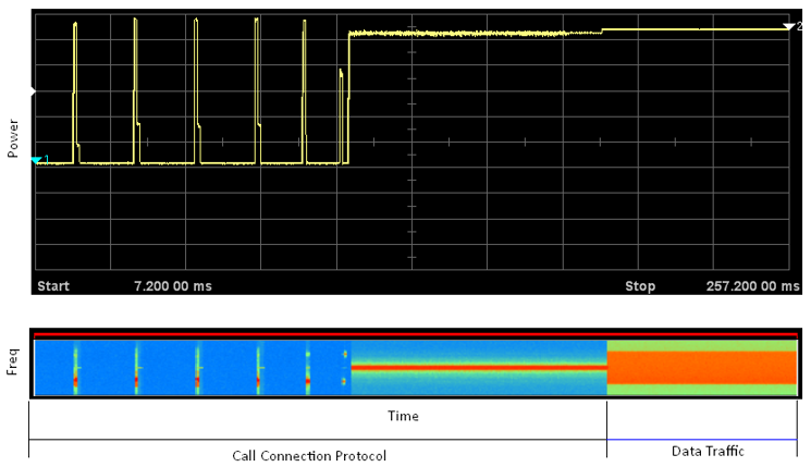
A quarter of a second of a real connection. The measurement problem is that the two halves need different instrument settings.

• The window is 250 ms : the upper pane runs from 7.200 00 ms to 257.200 00 ms with power on the vertical axis.
• The left part is a run of short isolated bursts : about five of them, each rising to a flat top and dropping back. That is the signalling before the connection is up.
• The right part is continuous : the trace steps up and stays there, with one further small step near the end of the window.
• The lower pane is a spectrogram : narrow coloured streaks line up with the early bursts, and a wide unbroken band covers the later part.
• The two regions are labelled underneath : Call Connection Protocol on the left and Data Traffic on the right.
• The occupied bandwidth widens with the traffic : the streaks are thin and the sustained band is broad. So the allocation grows once there is data to carry.

What is the implication of these multiple system bandwith and dynamic bandwidth change to Mobile phone designer and the test engineer ? For designers, the biggest issues would be how to optimize various kinds of design parameters to be best fit for all of these bands. For test engineers, the biggest issue would be huge number of the test cases they have to go through.

Final outcome of all these considerations on multiple bandwidth and dynamic bandwidth change can be examplified as a table shown below. This is a table for only one test case. See all those different system bandwith you have to cover. Different RB allocations is for dynamic frequency allocation that I mentioned above. In LTE, for every test case you would have this kind of tables and this will be huge headache to designers and test engineers.

The uplink half of the MPR test configuration. The downlink column is blank on purpose.

• The downlink is declared irrelevant : the Downlink Configuration column reads N/A for Maximum Power Reduction test case, so only what the UE sends matters.
• Four rows per channel bandwidth : QPSK and 16QAM, each at a partial allocation and at the full one.
• The larger number in each pair is the whole bandwidth : 6, 15, 25, 50, 75 and 100 resource blocks for 1.4, 3, 5, 10, 15 and 20 MHz.
• FDD and TDD are given the same allocations : the two columns carry identical numbers in every row.
• The initial conditions multiply the row count : five test environments and three frequency ranges apply to every row in the table.

LTE Specific Measurement

Even though LTE RF measurement has a lot of common characteristics which is similar to other technology, there are several measurement which is unique to LTE. Can you guess which would be the LTE specific tests ? If you recall unique properties of LTE signal that I described above, you would make a pretty good guess.

MPR - Maximum Power Reduction

Theoretically this test can be applied to UMTS as well, but as far as I know UMTS does not have this test as a formal conformance test item. It took me very long time to get some practical understanding on the purpose of this test. I didn't have clear understanding on how Maximum Power Reduction test is different from Maximum Output Power test. If you read test procedure of Maximum Output Power test and Maximum Power Reduction test, you would notice they are almost same. Actually there is no outstanding difference in terms of test procedure between Max Output Power test and Max Power Reduction test. The difference between the two lies in test condition and test requirement as illustrated below.

Max Output Power test is done with minimum modulation scheme (QPSK) and very small number of RB allocation. In Max Power Reduction test, we use more RB and higher modulation scheme comparing to Max Output Power test and then allow more margin (especially in negative side margin) in Max Power Reduction test.

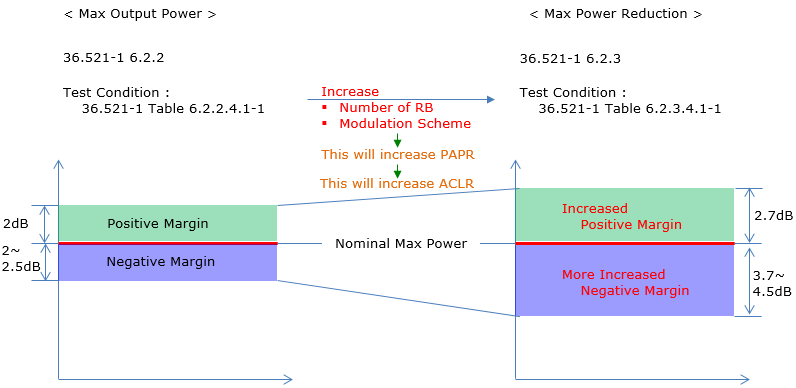
Two tests, one measurement, different windows. The arrow across the middle is the reason the window on the right is wider.

• The left block is 36.521-1 6.2.2 : its test condition is Table 6.2.2.4.1-1. Its window is 2 dB above the nominal maximum and 2 to 2.5 dB below it.
• The right block is 36.521-1 6.2.3 : its test condition is Table 6.2.3.4.1-1. Its window grows to 2.7 dB above and 3.7 to 4.5 dB below.
• The red line through both blocks is the same : Nominal Max Power does not move. So the two tests differ only in what they will accept around it.
• The middle of the drawing gives the chain : increasing the number of RB and the modulation scheme increases PAPR, and increasing PAPR increases ACLR.
• The window opens downward far more than upward : the positive margin grows by 0.7 dB and the negative margin by up to 2 dB. The UE answers a higher PAPR by reducing its power.

As described above, the test procedure is simple to understand .. do the same test as Max Output Power but just using different RB allocation and modulation scheme and apply relaxed passing condition(test requirement). The question is why we need to allow this kind of relaxation of the requirement when we increase the number of RB and Modulation scheme.

You may intuitively understand that PAPR (Peak to Average Power Ratio) will increase as the modulation depth increase (e.g, 16 QAM will produce larger PAPR than QPSK and 64 QAM will produce larger PAPR than 16 QAM). Also, if you are familiar with the property of OFDM, you would understand more RB (more sub carriers) will produce larger PAPR as well. In max power condition, the TX amplifier may operate at the very top of linear region. If you increase PAPR, the TX signal would easily goes into non-linear region of the amplifier and increase ACLR as result. One of the easiest way to prevent this kind of ACLR violation would be decrease the max power (max average power) a little bit. 3GPP decided to allow this kind max power reduction when the large number of RB is used or higher modulation scheme is used so that UE can lower the average max power a little bit to meet the ACLR passing criteria.

IBE - In-Band Emission

One of the most unique feature of LTE would be that in most case UE does not use full system bandwidth, meaning it uses only a portion of RF bandwidth. Just in terms of RF characteristics, this partial usage of RF band would not cause any serious problem, but what if the portion is allocated to only one side around the center frequency ? You would see the spectrum as follows.(I would not explain this picture in detail. Just take a close look and try to vervalize what you see in this picture and you would know the meaning and why we need to measure this item). The design goal for UE transmitter is to minimize the emission at the center frequency and the other emission (Image signal).

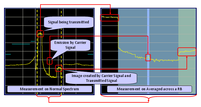
The same measurement twice. The right pane is what the specification actually checks, and averaging is what turns one into the other.

• The left pane is labelled Measurement on Normal Spectrum : a raw trace with two dashed markers, and three features called out on it.
• The right pane is labelled Measurement on Averaged across a RB : the same trace redrawn as a staircase, with one step per resource block.
• Three things are marked, and only one of them is wanted : Signal being transmitted, Emission by Carrier Signal, and Image created by Carrier Signal and Transmitted Signal.
• The red lines join each feature to its counterpart : every peak on the left has a step on the right. That is the point of putting the two panes side by side.
• Averaging is what makes a limit checkable : a spiky trace has no single value per block, and a staircase has exactly one.
• 36.101 keeps the carrier component separate : clause 6.5.2.2 is Carrier leakage and clause 6.5.2.3 is In-band emissions. So the two features the drawing names are two requirements.

Power Control - Absolute Power Tolerance

When UE transmit the first PUSCH, the power is determined by p0-NominalPUSCH and PUSCH Power Control Algorithm. This test is to check if UE set the accurate initial PUSCH power according to p0-NominalPUSCH and PUSCH Power Control Algorithm (This is different from what we call Open Loop Power Control in 3G. When we say "open loop power control", it usually mean the initial PRACH power. On the contrary, Absolute Power Tolerance is about the initial PUSCH power ).

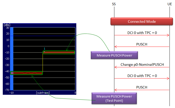
The closed loop is deliberately held at zero throughout. So the power step in the plot can only have come from the open loop.

• Both grants carry TPC = 0 : the sequence sends DCI 0 with TPC = 0 before the change and again after it. So the UE is never told to step its power.
• The only thing that changes is p0-NominalPUSCH : that message sits between the two grants and is the whole stimulus.
• The plot holds two flat levels : about -44 dBm and about -10 dBm, with a single step between them and no ramp.
• The vertical axis is dBm and the horizontal one is subframes : 30 down to -70 in 10 dB steps, over subframes -10 to 9.
• Two measurements are taken and the second is the test point : the first reading establishes where the UE was, and the second is the one judged.

Power Control - Relative Power Tolerance

Another aspect I want to mention is about power control. Overall power control test method is very similar to WCDMA ILPC(Inner Loop Power Control) test. Network (SS) sends a consecutive sequence of TPC command (Transmission Power Control command), like Up, Up, Up, Up... Down, Down, Down, Down,... and check if UE properly decode the command and set UE TX power indicated by each Up/Down command(+1 dB, -1 dB). LTE is using a similar method.. but if you see the following measurement you will see a huge jump in the middle which you didn't see with WCDMA. Does this mean that LTE has special TPC command like +10 dB jump or -10 dB fall ?

No. The big jump you see in the measurement is not as a result of big TPC command, but as a result of increase of number of RB. Even though UE transmit the same power at each subcarrier, the total power get larger if UE is using more subcarrier.

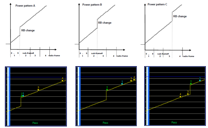
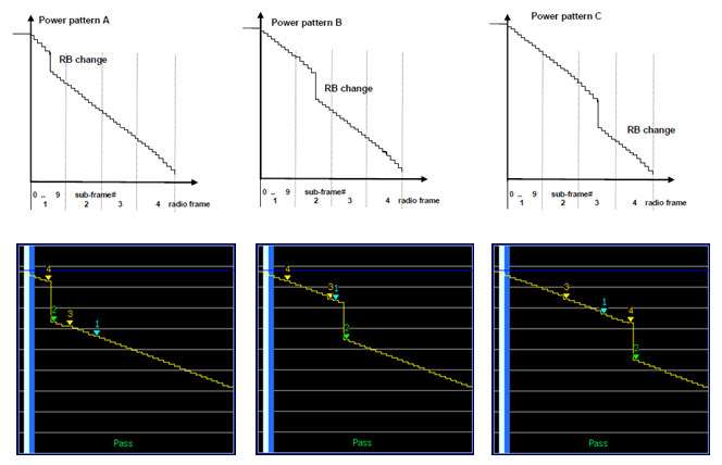
Six patterns in two pictures. The ramp goes up in one and down in the other, and the resource block change slides along it.

• Each picture holds three patterns labelled A, B and C : the upper row is the schematic and the lower row is the measurement that matches it.
• The ramp is a staircase, not a slope : the power moves one step per subframe. The axis underneath is marked in subframes and radio frames.
• What separates A from B from C is one vertical line : the line labelled RB change sits early, in the middle and late.
• The two pictures are mirror images : one ramps up across four radio frames and the other ramps down across the same span.
• All six measurements read Pass : the verdict is printed in green at the bottom of every lower plot.
• The discontinuity at the RB change is the thing being judged : a relative test asks about the size of each step. So the step that spans an allocation change is the hard one.

Aggregate Power Control Tolerance

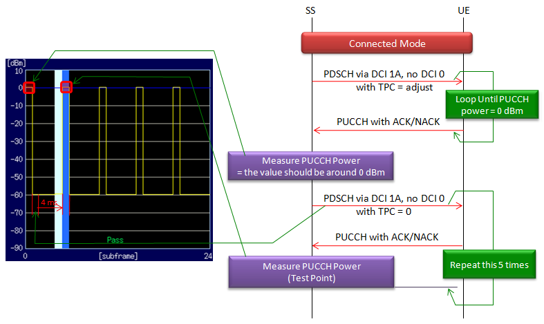
This test is to check how stably a UL power can maintained without any additional adjustment. This test is imporant because there are many situations during which UE cannot receive any power control command for adjustment like during measurement Gap or Connected Mode DRX.

Since this power stability should be applied both for PUCCH and PUSCH, this test is made up of two sub test, one for PUCCH and another one for PUSCH as illustrated below.

Following illustration is for PUCCH Aggregate Power Control Tolerance.

Following illustration is for PUSCH Aggregate Power Control Tolerance.

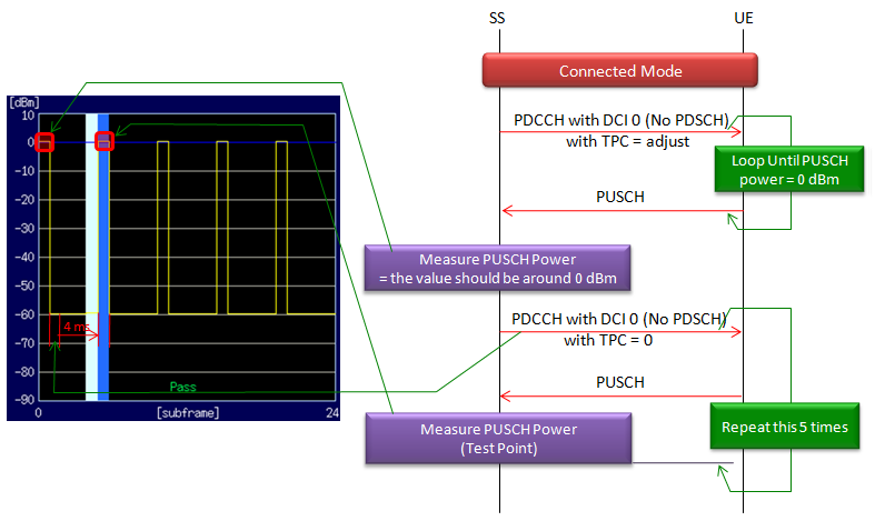
The same two phase shape for both uplink channels. Phase one gets the UE to a known power, and phase two measures what five commands of nothing add up to.

• Phase one walks the power to a known point : the TPC field is set to adjust and the loop runs until the measured power is 0 dBm.
• Phase two holds TPC = 0 and repeats five times : the UE is told to make no change five times over. The power after that is the test point.
• The two pictures differ in which channel is driven : the PUCCH case sends PDSCH via DCI 1A with no DCI 0. The PUSCH case sends PDCCH with DCI 0 and no PDSCH.
• The reply differs to match : PUCCH with ACK/NACK in one, and PUSCH in the other.
• Both plots show five bursts reaching about 0 dBm : the vertical axis runs 10 down to -90 dBm and the horizontal one covers subframes 0 to 24.
• The spacing is marked as 4 ms : a red annotation between the first two bursts gives it. That is the FDD gap between a downlink subframe and its uplink answer.
• Aggregate means the error is allowed to accumulate : five commands that each ask for no change should still leave the power where it was. This test measures how far it drifted.

• Four of these five tests are power measurements : only in-band emission needs the signal demodulated. The rest need a power reading at the right moment.
• MPR is not a separate measurement : it is the maximum power test with a wider window, run at allocations where the specification expects the UE to back off.
• Absolute, relative and aggregate ask three different questions : where the power landed, how big each step was. How far it drifted over a run of commands.
• The allocation is a test parameter everywhere here : it sets the PAPR that MPR allows for, it moves the emission the IBE test reads. It is the thing that changes mid ramp in the relative test.

RF Test Equipment/UE Connection Diagram

Following diagrams shows all the possible composition of test equipment and connections between the equipment and DUT(UE). You don't have to memorize all these diagrams. The main test description is in 36.521-1 and these diagram is in 36.508. So when you try to understand a test procedure you need to go back and forth between multiple documents. One of the main purpose of my note is to combine (consolidate) those multiple documents into one page, so that you can get the most of fundamental information for a test case from a single page.

But if you have some time or eagerness to understand deeply about RF conformance test case, examine these diagrams one by one and imange what kind of test can be done by each of these diagram (without looking into 36.521-1).

Also, understanding each of these diagram would be very helpful to troubleshoot the equipment when you are performing RF Conformance test. Most of the commercial RF conformance system is made up of many different equipments connected together. However, not all of the component equipment are used all together for every test cases. Each of the test cases would use a certain number of specific component equipment in the system.  When you come across a problem with a specific test cases and if you think the problem might be from the equipment (not from the UE), you may first check what kind of equipment configuration (one of the following diagrams) is used by the test case and check through the component equipment and connections in your RF conformance system.

< 36.508 Figure A.2: Connection for Transmitter Intermodulation tests >

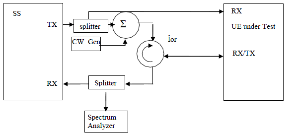
< 36.508 Figure A.3: Connection for basic single cell, RX and TX tests >

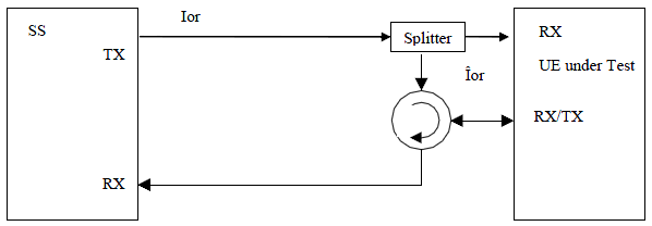
< 36.508 Alternative to Figure A.3 >

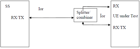
< 36.508 Figure A.4: Connection for Receiver tests with E-UTRA-Interference >

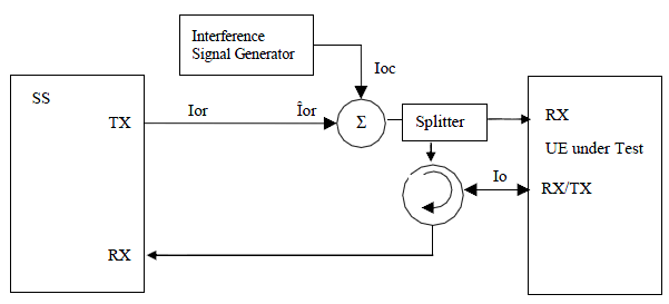
< 36.508 Figure A.5: Connection for Receiver tests with CW interferer >

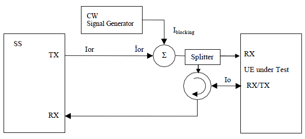
< 36.508 Figure A.6: Connection for Receiver tests with both E-UTRA Interference and additional CW signal >

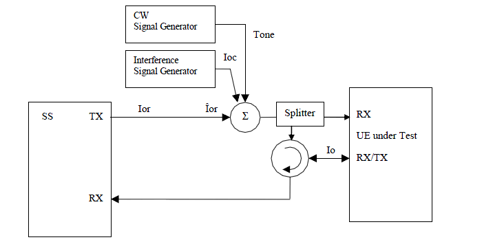
< 36.508 Figure Figure A.7: Connection for TX-tests with additional Spectrum Analyzer >

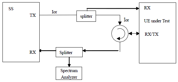
< 36.508 Figure A.8: Connection for RX-tests with additional Spectrum Analyzer >

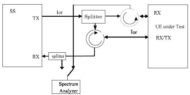
< 36.508 Figure A.9: Connection for RX performance tests with antenna configuration 1x2 (single antenna port) >

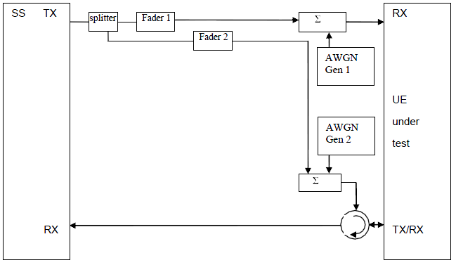
< 36.508 Figure A.10: Connection for RX performance tests with antenna configuration 2x2 >

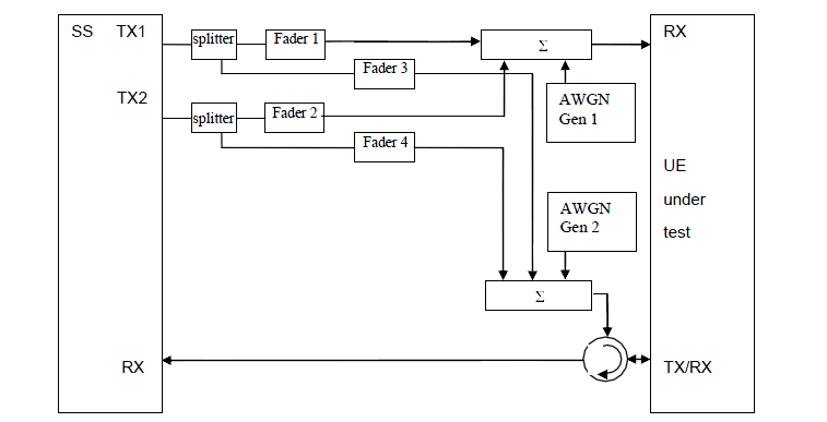
< 36.508 Figure A.11: Connection for RX performance tests with antenna configuration 4x2 >

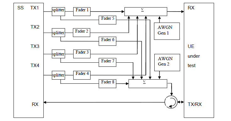
< 36.508 Figure A.14: Connection for 2 cells with static propagation and receive diversity >

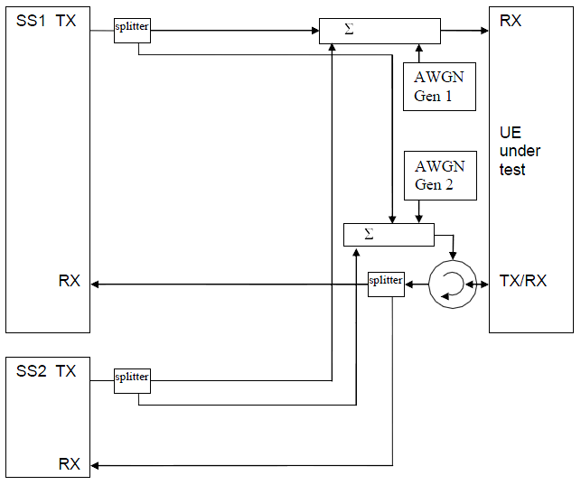
< 36.508 Figure A.15: Connection for 2 cells with multipath fading propagation and receive diversity >

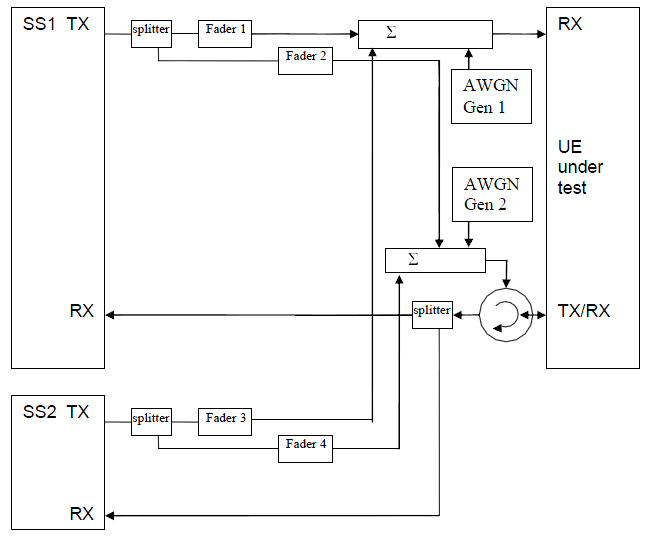
Thirteen drawings, and three questions separate them: how many simulators, how many faders, and what else is summed into the downlink.

• Figure A.3 is the one to learn first : one simulator transmit port reaches the UE receive port through a splitter, and the UE transmit and receive port through a circulator.
• Two labels do the bookkeeping : Ior is the level leaving the simulator, and the same symbol with a hat over it is the level arriving at the UE. Everything the splitters and the cables cost sits between the two.
• The alternative to A.3 uses one bidirectional port : a splitter combiner replaces the circulator. The same two labels appear on either side of it.
• Adding a generator is what makes a receiver test : A.4 sums an interference generator marked Ioc, A.5 sums a CW generator carrying the blocking level, and A.6 sums both.
• Io appears once there is something to add : it labels the total arriving at the UE, where the hatted Ior labels the wanted part of it.
• A spectrum analyser marks a transmitter test : A.7 taps the uplink return, A.2 adds a CW generator to the same arrangement, and A.8 puts a circulator on both UE ports.
• Faders count transmit antennas : A.9 has one transmit port and two faders, A.10 has two ports and four, and A.11 has four ports and eight.
• Two simulators mean two cells : A.14 combines SS1 and SS2 with no faders at all, and A.15 is the same pair with four faders between them.
• Two AWGN generators appear in every faded diagram : one per receive branch. That is what makes the noise independent on the two UE antennas.

• Read the extra boxes, not the wiring : the splitters and circulators are the same in nearly every drawing. What changes is what is summed in.
• A fader means a performance test : the demodulation tests need a channel model, and nothing in chapters 6 or 7 does.
• The number of faders is transmit ports times two : two receive branches are assumed throughout, so eight faders means four transmit antennas.
• The label chain is worth learning once : Ior at the simulator, the hatted Ior at the UE, Ioc for interference and Io for the total.

Protocol Sequence for RF Conformance Test

The overall protocol sequence for RF conformance test is defined in 36.508. But most of the equipment vendor put a little variation. I put one example sequence below.

1) MIB

2) SIB 1, 2, 3

3) RRC : PRACH Preamble

4) RRC : RACH Response

5) RRC : RRC Connection Request

6) RRC : RRC Connection Setup

7) RRC : RRC Connection Setup Complete + NAS : Attach Request

8) RRC : DL Information Transfer + NAS : Authentication Request

9) RRC : UL Information Transfer + NAS : Authentication Response

10) RRC : DL Information Transfer + NAS : Security Mode Command

11) RRC : UL Information Transfer + NAS : Security Mode Complete

12) RRC: DLInformationTransfer + TC: ACTIVATE TEST MODE

13) RRC: ULInformationTransfer + TC: ACTIVATE TEST MODE COMPLETE

14) RRC : Security Mode Command

15) RRC : Security Mode Complete

16) RRC: UECapabilityEnquiry

17) RRC: UECapabilityInformation

15) RRC : RRC Connection Reconfiguration + NAS : Attach Accept + NAS : Activate Default EPS Bearer Context Req

16) RRC : RRC Connection Reconfiguration Complete + NAS : Attach Complete

17) RRC : RRC Connection Release

< MO or MT call > : In MT call, Paging should be sent.

18) RRC : PRACH Preamble

19) RRC : RACH Response

20) RRC : RRC Connection Request

21) RRC : RRC Connection Setup

22) RRC : RRC Connection Setup Complete

23) RRC : Security Mode Command

24) RRC : Security Mode Complete

25) RRC : RRC Connection Reconfiguration

26) RRC : RRC Connection Reconfiguration Complete

< Perform Test Case >

27) RRC : RRC Connection Release

One important step and major different part from the ordinary call processing protocol sequence is "TC: ACTIVATE TEST MODE". This part is described in detail in the following specifications.

36.509 - 6.5 ACTIVATE TEST MODE

36.509 - 5.3.2.3 Reception of ACTIVATE TEST MODE message by UE

Unlike the test mode in UMTS, LTE test mode in RF conformance testing does not establish the loopback mode. The main purpose of the test mode in LTE described in the 36.509 - 5.3.2.3 as follows.

When the UE test mode is active, the UE shall accept any request to establish a data radio bearer with an associated EPS bearer context, both included in the same RRC message, and within the radio access capabilities of the UE.

Two things about the list above matter before the next section. It covers two connections rather than one, and its step numbers restart partway down.

• The sequence runs two connection cycles : the first carries the attach and ends in an RRC Connection Release. The second is the one the test case runs in.
• The step numbers repeat : 15, 16 and 17 appear twice, once for the security and capability exchange and again for the reconfiguration and release. Read the list by its message names rather than by its numbering.
• Only two steps are specific to a test : ACTIVATE TEST MODE and its COMPLETE, carried in DLInformationTransfer and ULInformationTransfer.
• Test mode is not loopback mode : 36.509 clause 6.5 carries a UE test loop mode element in ACTIVATE TEST MODE. Its note says no specific UE action is currently specified on receiving it.
• The second cycle is where the measurement happens : everything before the MO or MT call is setup. That is why a failing RF test is often a failing attach.

RF Conformance Test - TRX Conformance - 36.521-1

It seems that many people think RF conformance is only for testing the performance/functionality of RF front end part of the mobile phone. It may be true, but eventual purpose of these test is to make sure that UE is functioning without any problem in live network. So each of these test items are related to one or more procedure happening in live network.

Therefore, it is very important to have big picture of live network procedures happenning between UE and the network and to find correlation between these conformance test items and the step/steps of live network process.

Often people ask me "Why we need to test these test items ? What is the purpose of these test ?". If you see the 3GPP specification (36.521) to find answers to these queston.. the answer is described as follows under 'test purpose' section.

Following example is for 6.3 Output Power Dynamics.

To verify the UE's ability to transmit with a broadband output power below the value specified in the test requirement when the power is set to a minimum value

Does this make any sense to you ? Not much to me at least. This description is good for test/pass-fail criterial, but does not give me any practical meaning for the test purpose.

My recommendation is to describe the overall live network procedure at very high level as follows and try to map each of the conformance test cases to the steps of your high level description.

i) UE is Off

ii) Power On UE

iii) < Frequency Search >

iv) < Cell Search > : Normally a UE would find multiple cells in this process

v) < Cell Selection >

vi) MIB decoding

vii) SIB deconding

viii) < Initial RACH Process >

ix) < Registration/Authentication/Attach>

x) <Default EPS Bearer Setup >

xi) Now UE is in IDLE Mode

xi) <(If the current cell become weak or UE moves to another cell regisn) Cell Reselection>

xii) <(When Paging message comes or User make a call) RACH Process>

xiii) < Setup Dedicated EPS Bearer >

xiv) Receive data

xv) Transmit data

xvi)  (If UE power is percieved too weak by the network) Network send TPC command to increase UE Tx Power

xvii) (If UE power is percieved too strong by the network) Network send TPC command to decrease UE Tx Power

xviii) < (If UE moves to another cell region) Network and UE perform Handover procedure >

xix) User stop call and UE gets into IDLE mode

If you just blindly looking into conformance test specification, you may be overwhelmed by the number of test cases. Would it be possible for me to understand all of these ? Do I have to give up digging into the details and just press button on the test system and take blindly whatver the machine spits out ?

But once you get the big pictures of these test cases, you will notice that all of those test cases can be grouped into only handfull of framework.

My recommendation for you is to try to understand the concept (big picture) of each chapter first rather than directly jumping into each of the test cases.

Let's take look at each chapters of TRX conformance 36.521-1. These four chapters are related to the whole procedure described above except iii), v), xviii).

Chapter 6, 7 is straightforward and they are most widely tested from the development stage even at manufacturing line. You may get a little bit confused by the title of the chapter 8. When we say "Performance", many people would think of "IP throughput". But in this case it is not true. "Performance" in this case means "How well a UE can successfully decode downlink signal even under various noisy channel condition". Chapter 9 is to measure "How accurately UE measure various channel condition and report to the network ?". In short, it is measuring CQI (Channel Quality Indicator), RI (Rank Index) , PMI (Precoding Matrix Index).

Chapter	Test Category
6	Transmitter Characteristics
7	Receiver Characteristics
8	Performance Requirement
9	Reporting of Channel State Information

Now let's look into each test cases in each chapter. Chapter 6 (Transmitter Characteristic) has following test cases. As you see, it is just measuring UE transmission power in various condition and data modulation quality. Most of the test items that is uniq to LTE are in this group, for example,

Chapter 6	Transmitter Characteristics - Measurement Items
6.2.2	Transmit power / UE Maximum Output Power
6.2.3	Transmit power / Maximum Power Reduction (MPR)
6.2.4	Transmit power / Additional Maximum Power Reduction (A-MPR)
6.2.5	Transmit power / Configured UE transmitted Output Power
6.3.2	Output Power Dynamics / Minimum Output Power
6.3.4.1	Output Power Dynamics / ON/OFF time mask / General ON/OFF time mask
6.3.4.2.1	Output Power Dynamics / PRACH and SRS time mask / PRACH time mask
6.3.4.2.2	Output Power Dynamics / PRACH and SRS time mask / SRS time mask
6.3.5.1	Output Power Dynamics / Power Control / Power Control Absolute power tolerance
6.3.5.2	Output Power Dynamics / Power Control / Power Control Relative power tolerance
6.3.5.3	Output Power Dynamics / Power Control / Aggregate power control tolerance
6.5.1	Transmit signal quality / Frequency Error
6.5.2.1	Transmit signal quality / Transmit modulation / Error Vector Magnitude (EVM)
6.5.2.1A	Transmit signal quality / Transmit modulation / PUSCH-EVM with exclusion period
6.5.2.2	Transmit signal quality / Transmit modulation / Carrier leakage
6.5.2.3	Transmit signal quality / Transmit modulation /  In-band emissions for non allocated RB
6.5.2.4	Transmit signal quality / Transmit modulation / EVM equalizer spectrum flatness
6.6.1	Output RF spectrum emissions / Occupied bandwidth
6.6.2.1	Output RF spectrum emissions / Out of band emission / Spectrum Emission Mask
6.6.2.3	Output RF spectrum emissions / Out of band emission / Adjacent Channel Leakage power Ratio
6.6.3.1	Output RF spectrum emissions / Spurious emissions / Transmitter Spurious emissions
6.6.3.2	Output RF spectrum emissions / Spurious emissions / Spurious emission band UE co-existence
6.6.3.3	Output RF spectrum emissions / Spurious emissions / Additional spurious emissions
6.7	Transmit intermodulation

Chapter 7 is almost identical to WCDMA reciever measurement. Basically all of these test cases measures how much data is properly decoded and how much data get lost under various UE reciever power (network transmission power).

Chapter 7	Receiver Characteristics - Measurement Items
7.3	Reference sensitivity level
7.4	Maximum input level
7.5	Adjacent Channel Selectivity (ACS)
7.6.1	Blocking characteristics / In-band blocking
7.6.2	Blocking characteristics / Out of-band blocking
7.6.3	Blocking characteristics / Narrow band blocking
7.7	Spurious response
7.8.1	Intermodulation characteristics / Wide band Intermodulation
7.9	Spurious emissions

Chapter 8 test mostly about how well UE can demodulate the important downlink signal (e.g, PDSCH, PCFICH/PDCCH, PHICH) under various noisy/fading channel condition. As you may guess, these test cases is using test system configuration like A9, A10, A11 as shown in previous section (TS 36.508 Annex A).

Chapter 8	Performance Requirement - Measurement Items
8.2.1.1.1	Demodulation of PDSCH (Cell-Specific Reference Symbols) / FDD (Fixed Reference Channel) / FDD PDSCH Single Antenna Port Performance (Cell-Specific Reference Symbols) / FDD PDSCH Single Antenna Port Performance
8.2.1.1.2	Demodulation of PDSCH (Cell-Specific Reference Symbols) / FDD (Fixed Reference Channel) / FDD PDSCH Single Antenna Port Performance (Cell-Specific Reference Symbols) / FDD PDSCH Single Antenna Port Performance with 1PRB
8.2.1.2.1	Demodulation of PDSCH (Cell-Specific Reference Symbols) / FDD (Fixed Reference Channel) / FDD PDSCH Transmit Diversity Performance (Cell-Specific Reference Symbols) / FDD PDSCH Transmit Diversity 2x2
8.2.1.3.1	Demodulation of PDSCH (Cell-Specific Reference Symbols) / FDD (Fixed Reference Channel) / FDD PDSCH Open Loop Spatial Multiplexing Performance (Cell-Specific Reference Symbols) / FDD PDSCH Open Loop Spatial Multiplexing 2x2
8.2.1.3.2	Demodulation of PDSCH (Cell-Specific Reference Symbols) / FDD (Fixed Reference Channel) / FDD PDSCH Open Loop Spatial Multiplexing Performance (Cell-Specific Reference Symbols) / FDD PDSCH Open Loop Spatial Multiplexing 4x2
8.2.1.4.1	Demodulation of PDSCH (Cell-Specific Reference Symbols) / FDD (Fixed Reference Channel) / FDD PDSCH Closed Loop Spatial Multiplexing Performance (Cell-Specific Reference Symbols) / FDD PDSCH Closed Loop Single/Multi Layer Spatial Multiplexing 2 x 2
8.2.1.4.2	Demodulation of PDSCH (Cell-Specific Reference Symbols) / FDD (Fixed Reference Channel) / FDD PDSCH Closed Loop Spatial Multiplexing Performance (Cell-Specific Reference Symbols) / FDD PDSCH Closed Loop Single/Multi Layer Spatial Multiplexing 4 x 2
8.4.1.1	Demodulation of PCFICH/PDCCH / FDD / FDD PCFICH/PDCCH Single-antenna Port Performance
8.4.1.2.2	Demodulation of PCFICH/PDCCH / FDD / FDD PCFICH/PDCCH Transmit Diversity Performance / FDD PCFICH/PDCCH Transmit Diversity 4x2
8.5.1.1	Demodulation of PHICH / FDD / FDD PHICH Single-antenna Port Performance
8.5.1.2.2	Demodulation of PHICH / FDD / FDD PHICH Transmit Diversity Performance / FDD PHICH Transmit Diversity 4x2

Chapter 9 is for measuring various feedback from UE regarding the radio channel quality (CQI, RI, PMI). For this measurement, we have to emulate various channel condition, so we need to use test configuration like A9, A10 etc as shown in previous section (TS 36.508 Annex A)

Chapter 9	Reporting of Channel State Information - Measurement Items
9.2.1.1	CQI Performance under AWGN conditions / CQI Reporting under AWGN conditions - PUCCH 1-0 / FDD CQI Reporting under AWGN conditions - PUCCH 1-0
9.2.2.1	CQI Performance under AWGN conditions / CQI Reporting under AWGN conditions - PUCCH 1-1 / FDD CQI Reporting under AWGN conditions - PUCCH 1-1
9.3.1.1.1	CQI Reporting under fading conditions / Frequency-selective scheduling mode / Frequency-selective scheduling mode - PUSCH 3-0 / FDD Frequency-selective scheduling mode - PUSCH 3-0
9.3.2.1.1	CQI Reporting under fading conditions / Frequency non-selective scheduling mode / Frequency non-selective scheduling mode - PUCCH 1-0 / FDD Frequency non-selective scheduling mode - PUCCH 1-0
9.3.3.1.1	CQI Reporting under fading conditions / Frequency-selective interference / Frequency-selective scheduling mode - PUSCH 3-0 / FDD Frequency-selective scheduling mode - PUSCH 3-0
9.4.1.1.1	Reporting of Precoding Matrix Indicator (PMI) / Single PMI / Single PMI - PUSCH 3-1 / FDD Single PMI - PUSCH 3-1
9.4.2.1.1	Reporting of Precoding Matrix Indicator (PMI) / Multiple PMI / Multiple PMI - PUSCH 1-2 / FDD Multiple PMI - PUSCH 1-2
9.5.1.1	Reporting of Rank Indicator (RI) / RI Reporting - PUCCH 1-1 / FDD RI Reporting- PUCCH 1-1

RF Conformance Test - RRM Conformance - 36.521-3

Radio resource management is tested in a separate document from the radio itself, and the reason is the stopwatch. Almost nothing in 36.521-3 is a level or a ratio. What is measured is how long the UE takes to do something, and how often it gets it right.

Chapter	Test Category
4	E-UTRAN RRC_IDLE State Mobility
5	E-UTRAN RRC_CONNECTED State Mobility
6	RRC Connection Mobility Control
7	Timing and Signalling Characteristics
8	UE Measurements Procedures
9	Measurement Performance Requirements

Chapter 4	E-UTRAN RRC_IDLE State Mobility - Measurement Items
4.2.1	E-UTRAN Cell Re-Selection / E-UTRAN FDD - FDD cell re-selection intra frequency case
4.2.3	E-UTRAN Cell Re-Selection / E-UTRAN FDD - FDD cell re-selection inter frequency case
4.3.1.1	E-UTRAN to UTRAN Cell Re-Selection / E-UTRAN FDD - UTRAN FDD cell re-selection / E-UTRA FDD-UTRAN FDD cell reselection: UTRA FDD is of higher priority
4.3.1.2	E-UTRAN to UTRAN Cell Re-Selection / E-UTRAN FDD - UTRAN FDD cell re-selection / E-UTRA FDD-UTRAN FDD cell re-selection: UTRA FDD is of lower priority
4.3.1.3	E-UTRAN to UTRAN Cell Re-Selection / E-UTRAN FDD - UTRAN FDD cell re-selection / E-UTRAN FDD - UTRAN FDD cell re-selection in fading propagation conditions: UTRA FDD is of lower priority
4.4.1	E-UTRAN to GSM Cell Re-Selection / E-UTRAN FDD - GSM cell re-selection

Chapter 5	E-UTRAN RRC_CONNECTED State Mobility - Measurement Items
5.1.1	E-UTRAN Handover / E-UTRAN FDD-FDD Handover intra frequency case
5.1.3	E-UTRAN Handover / E-UTRAN FDD-FDD Handover inter frequency case
5.1.5	E-UTRAN Handover / E-UTRAN FDD-FDD inter frequency Handover: unknown target cell
5.2.1	Handover from E-UTRAN to other RATs / E-UTRAN FDD - UTRAN FDD handover
5.2.3	E-UTRAN to UTRAN Cell Re-Selection / E-UTRAN FDD - UTRAN FDD cell re-selection / E-UTRAN FDD - UTRAN FDD cell re-selection in fading propagation conditions: UTRA FDD is of lower priority
5.2.7	Handover from E-UTRAN to other RATs / E-UTRAN FDD - UTRAN FDD handover: unknown target cell
5.2.8	Handover from E-UTRAN to other RATs / E-UTRAN FDD - GSM handover: unknown target cell

Chapter 6	RRC Connection Mobility Control - Measurement Items
6.1.1	RRC Re-establishment / E-UTRAN FDD Intra-frequency RRC Re-establishment
6.1.2	RRC Re-establishment / E-UTRAN FDD Inter-frequency RRC Re-establishment
6.2.1	Random Access / E-UTRAN FDD - Contention Based Random Access Test
6.2.2	Random Access / E-UTRAN FDD - Non-Contention Based Random Access Test

Chapter 7	Timing and Signalling Characteristics - Measurement Items
7.1.1	UE Transmit Timing / E-UTRAN FDD - UE Transmit Timing Accuracy
7.2.1	UE Timing Advance / E-UTRAN FDD - UE Timing Advance Adjustment Accuracy
7.3.1	UE Transmit Timing / E-UTRAN FDD Radio Link Monitoring Test for Out-of-sync
7.3.2	UE Transmit Timing / E-UTRAN FDD Radio Link Monitoring Test for In-sync
7.3.5	UE Transmit Timing / E-UTRAN FDD Radio Link Monitoring Test for Out-of-sync in DRX
7.3.6	UE Transmit Timing / E-UTRAN FDD Radio Link Monitoring Test for In-sync in DRX

Chapter 8	UE Measurements Procedures- Measurement Items
8.1.1	E-UTRAN intra frequency measurements / E-UTRAN FDD intra frequency measurements / E-UTRAN FDD-FDD intra frequency event triggered reporting under fading propagation conditions in asynchronous cells
8.1.2	E-UTRAN intra frequency measurements / E-UTRAN FDD intra frequency measurements / E-UTRAN FDD-FDD intra frequency event triggered reporting under fading propagation conditions in synchronous cells
8.1.3	E-UTRAN intra frequency measurements / E-UTRAN FDD intra frequency measurements / E-UTRAN FDD-FDD intra frequency event triggered reporting under fading propagation conditions in synchronous cells with DRX
8.3.1	E-UTRAN FDD-FDD Inter-frequency Measurements / E-UTRAN FDD-FDD Inter-frequency event triggered reporting under fading propagation conditions in asynchronous cells
8.3.2	E-UTRAN FDD-FDD Inter-frequency Measurements / E-UTRAN FDD-FDD Inter-frequency event triggered reporting when DRX is used under fading propagation conditions in asynchronous cells
8.3.3	E-UTRAN FDD-FDD Inter-frequency Measurements / E-UTRAN FDD-FDD Inter frequency event triggered reporting under AWGN propagation conditions in asynchronous cells with DRX when L3 filtering is used
8.5.1	E-UTRAN FDD - UTRAN measurements / E-UTRAN FDD - UTRAN FDD event triggered reporting under fading propagation conditions
8.5.2	E-UTRAN FDD - UTRAN measurements / E-UTRAN FDD - UTRAN FDD SON ANR cell search reporting under AWGN propagation conditions
8.5.3	E-UTRAN FDD - UTRAN measurements / E-UTRAN FDD - UTRAN FDD event triggered reporting when DRX is used under fading propagation conditions
8.8.1	E-UTRAN FDD - GSM measurements / E-UTRAN FDD - GSM event triggered reporting in AWGN
8.8.2	E-UTRAN FDD - GSM measurements / E-UTRAN FDD - GSM event triggered reporting when DRX is used in AWGN
8.11.1	Monitoring of Multiple Layers / Multiple E-UTRAN FDD-FDD Inter-frequency event triggered reporting under fading propagation conditions
8.11.3	Monitoring of Multiple Layers / E-UTRAN FDD-FDD Inter-frequency and UTRAN FDD event triggered reporting under fading propagation conditions
8.11.5	Monitoring of Multiple Layers / Combined E-UTRAN FDD - E-UTRA FDD and GSM cell search. E-UTRA cells in fading; GSM cell in static propagation conditions

Chapter 9	Measurement Performance Requirements - Measurement Items
9.1.1.1	RSRP / FDD Intra frequency RSRP Accuracy / FDD Intra Frequency Absolute RSRP Accuracy
9.1.1.2	RSRP / FDD Intra frequency RSRP Accuracy / FDD Intra Frequency Relative Accuracy of RSRP
9.1.3.1	RSRP / FDD Inter frequency RSRP Accuracy / FDD - FDD Inter Frequency Absolute RSRP Accuracy
9.1.3.2	RSRP / FDD Inter frequency RSRP Accuracy / FDD - FDD Inter Frequency Relative Accuracy of RSRP
9.2.1.1	RSRQ / FDD Intra frequency RSRQ Accuracy / FDD Intra Frequency Absolute RSRQ Accuracy
9.2.3.1	RSRQ / FDD - FDD Inter frequency RSRQ Accuracy / FDD - FDD Inter Frequency Absolute RSRQ Accuracy
9.2.3.2	RSRQ / FDD - FDD Inter frequency RSRQ Accuracy / FDD - FDD Inter Frequency Relative Accuracy of RSRQ

Overview on RF/PHY Performance Test

Basic Idea of Performance Test for RF/PHY is pretty simple. As you see in the following diagram, a DUT (UE) is connected to SS (Signaling Simulator) with single cell and Fader and AWGN are connected to the downlink path of the connection.

The purpose is to test how well UE can decode various downlink physical channels under harsh channel condition (e.g, in the exisitance of AWGN and/or Fading).

The connection that defines a performance test. A fader on each branch and its own noise source is what separates this from a receiver test.

• One simulator transmit port feeds two branches : a splitter sends it to Fader 1 and Fader 2.
• Each branch gets its own noise : Fader 1 is summed with AWGN Gen 1 and Fader 2 with AWGN Gen 2, at separate summing points.
• The two branches land on different UE ports : one on the RX port and the other through a circulator on the TX/RX port.
• The uplink comes back through that circulator : the UE answer reaches the simulator receive port on the same cable as the second downlink branch.
• Independent faders are the whole idea : receive diversity only exists when the two branches fade differently. Two faders are how a bench creates that.

• A performance test measures throughput, not a level : the UE is given a defined channel and a defined noise level. What is judged is how much data survives.
• The fading condition is a test parameter like any other : EVA5, ETU70, ETU300 and HST each stand for a delay profile and a Doppler rate.
• Rho A, Rho B and Noc set the working point : two power ratios and a noise density. Together they fix the signal to noise ratio the UE has to work at.
• The connection diagram tells you the test class : if the drawing has faders in it, the test is in chapter 8.

You can find the details of the performance test from 36.521-1 8 Performance Requirement. There are pretty many test cases under this chapter as in the table in previous section but we can simplify the whole set of test in a simple table as follows.

Four rows is a small table for a chapter this size, and that is the useful part. Every performance test in 36.521-1 chapter 8 is a choice of one entry from each row.

• The channel row is not all data : PDSCH, PCFICH/PDCCH, PBCH and PHICH, so half of it is control and broadcast.
• Finding the grant is tested as hard as decoding the payload : a UE that cannot read PCFICH and PDCCH never reaches PDSCH. Each of the three has its own test.
• The parameter row is two power ratios, a noise level and a modulation : Rho A, Rho B, Noc and the modulation scheme, which together fix the working point.
• The fading names carry a profile and a Doppler figure : EVA5, ETU70 and ETU300 share a profile letter group with a different number, and HST is the high speed case.
• The SNR row runs from -1.0 to 19.1 : a span of about 20 dB, and the low end sits below zero.
• Below zero means the wanted signal is weaker than the noise : those are the tests that decide whether a UE holds a call at the edge of a cell.

Note : If you are interested in more exhaustive test, refer to Physical Layer Throughput/Performance Test (My personal test)

Test Case Description

In this section, I will describe some of the test cases that are most commonly tested (It would not be possible (it wouldn't have much meaning) to describe all the test cases. I will just pick some of them and describe it in my own words.

36.521-1 : 6.2.2 UE Maximum Output Power

As the test case title implies, this test case is to measure UE Max Tx power. This would be the most basic test cases for almost everybody would check at first.

Procedure :

The precedure description here would not map one-to-one to 3GPP descrition. The way I describe here is the combined procedure of "Initial Condition" and "Test Procedure" section of 3GPP. I think the description here would be easier to understand (at least to me :))

Step 1 : Connect the equipment and UE as follows.

< 36.508 Figure A.3: Connection for basic single cell, RX and TX tests >

Step 2 : Configure Downlink Power as shown below. As you see here the total channel power varies depending on Channel Bandwidth, but RS EPRE is same in any case.

< 36.521-1 Table C.0-1: Default Downlink power levels >

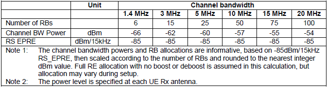
One downlink level for every channel bandwidth, all derived from a single figure by arithmetic.

• RS EPRE is the same in every column : -85 dBm per 15 kHz. That is the one number the rest of the row is built from.
• The resource block counts are the standard ones : 6, 15, 25, 50, 75 and 100 for 1.4, 3, 5, 10, 15 and 20 MHz.
• Channel bandwidth power is RS EPRE scaled by the subcarrier count : 6 blocks is 72 subcarriers, which adds 18.6 dB to -85 and rounds to the -66 dBm printed.
• The same sum gives every other column : 300 subcarriers gives -60.2, 600 gives -57.2 and 1200 gives -54.2, matching the -60, -57 and -54 in the table.
• Note 1 says the values are informative : full resource element allocation with no boost or deboost is assumed, and the allocation may vary during setup.
• Note 2 places the measurement : the power level is specified at each UE receive antenna, not at the simulator output.

The more detailed parameters for other physical channels are specified in 36.521-1 Table C.1-1, Table C.3.0-1, Table C.3.0-2, Table C.3.0-3, but I will not copy those tables here since it is not so important on understanding the concept of the test cases.   

Step 3 : Configure UL RB as shown below. As you see here, you don't set the max number of RB (Full RB) here, you will allocate only a portion of the channel bandwidth (Partial RB). The definition of partial RB (i.e, how many RBs should be used) is defined in following table.

< 36.521-1 Table 6.2.2.4.1-1: Test Configuration Table >

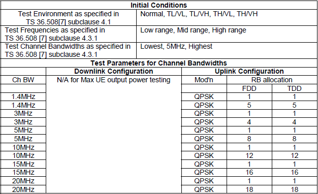
Compare the allocations here with the MPR table earlier on the page. The difference between the two tables is the whole difference between the two tests.

• QPSK only, and two rows per channel bandwidth : one resource block, then a partial allocation of 5, 4, 8, 12, 16 or 18 blocks.
• The full allocation never appears : the largest entry is 18 blocks of the 100 available at 20 MHz.
• That is what separates this test from the MPR test : the MPR table runs the same bandwidths at 100 blocks and at 16QAM. Those are the conditions where the UE may reduce its power.
• The partial allocations match the MPR table exactly : 5, 4, 8, 12, 16 and 18 appear as the smaller of the two allocations there.
• Three channel bandwidths, not four : Lowest, 5MHz and Highest, where the MPR table adds 10MHz.
• The downlink is again N/A : nothing about the downlink affects how much power the UE may transmit.

Other detailed parameters like MCS should be inferenced by referring to following table.

< 36.521-1 Table A.2.2.2.1-1: Reference Channels for QPSK with partial RB allocation >

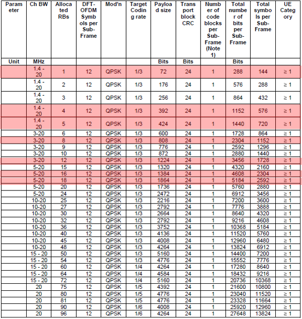
The reference channels behind those allocations. Every highlighted row is one the maximum output power test uses.

• The highlighted rows are 1, 4, 5, 8, 12, 16 and 18 resource blocks : exactly the allocations the test configuration table above asks for.
• Twelve DFT-OFDM symbols per subframe in every row : fourteen symbols less the two the demodulation reference signal takes, one per slot.
• The symbol count is the block count times 144 : one block gives 144 symbols, four gives 576 and eighteen gives 2592.
• The bit count is twice that, because the modulation is QPSK : 288, 1152 and 5184 bits per subframe for those same three rows.
• The target coding rate is 1/3 and the table holds to it : 72 payload bits plus 24 CRC over 288 is exactly a third. The 18 block row gives 1888 over 5184, which is 0.364.
• The CRC is 24 bits in every row : one transport block per subframe, so one CRC.

For further information about other Uplink physical channel is specified in Table H.1-1, Table H.1-2. but I will not copy those tables here since it is not so important on understanding the concept of the test cases.

Step 4 :  Start the test case in the test equipment (SS), power on DUT and get the DUT in connection (communication) with the SS. The equipment send DCI 0 (UL Grant) for every subframe that make UE to transmit PUSCH every subframe.

Step 5 : Equipment (SS) should send TPC UP command for at least 200 ms to get UE Tx power reach to the max power.

Step 6 : Measure the UE Tx power across the channel bandwidth (at least for one subframe).

36.521-1 : 7.3 Reference sensitivity level

The precedure description here would not map one-to-one to 3GPP descrition. The way I describe here is the combined procedure of "Initial Condition" and "Test Procedure" section of 3GPP.

Step 1 : Connect the equipment and UE as follows.

< 36.508 Figure A.3: Connection for basic single cell, RX and TX tests >

Step 2 : Configure Downlink Power as shown below. As you see here the total channel power varies depending on Channel Bandwidth, but RS EPRE is same in any case.

< 36.521-1 Table C.0-1: Default Downlink power levels >

The more detailed parameters for other physical channels are specified in 36.521-1 Table C.1-1, Table C.3.0-1, Table C.3.0-2, Table C.3.0-3, but I will not copy those tables here since it is not so important on understanding the concept of the test cases.   

Step 3 : Configure UL RB as shown below. As you see here, you don't set the max number of RB (Full RB) here, you will allocate only a portion of the channel bandwidth (Partial RB). The definition of partial RB (i.e, how many RBs should be used) is defined in following table.

< 36.521-1 Table 7.3.4.1-1: Test Configuration Table >

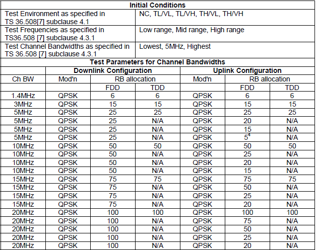
The downlink is held at full allocation in every row. What the table sweeps is the uplink, and the TDD column shows why.

• The downlink allocation is always the whole bandwidth : 6, 15, 25, 50, 75 or 100 resource blocks, QPSK, in every row.
• The uplink allocation is what varies : 20 MHz alone is listed at 100, 75, 50, 25 and 20 blocks.
• Every reduced uplink row has N/A in the TDD column : those rows exist only for FDD.
• That asymmetry is the point of the test : only an FDD UE transmits and receives at the same instant. So only an FDD UE desensitises its own receiver.
• Both directions are configured here : the transmitter test tables left the downlink column N/A, and this one cannot.
• The test environment row reads NC rather than Normal : the four extreme corners TL/VL, TL/VH, TH/VL and TH/VH are the same as in the transmitter tables.

Step 4 :  Start the test case in the test equipment (SS), power on DUT and get the DUT in connection (communication) with the SS.

Step 5 : The equipment send DCI 1A and PDSCH for every subframe.

Step 6 : The equipment send DCI 0 (UL Grant) for every subframe that make UE to transmit PUSCH every subframe.

Step 7 : Equipment (SS) set the downlink power as shown below and should send TPC UP command to get UE Tx power reach to the max power. As you see, the dowlink power varies depending Channel Bandwidth and Band.

< 36.521-1 Table 7.3.5-1: Reference sensitivity QPSK P_REFSENS >

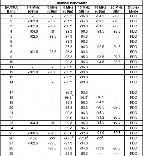
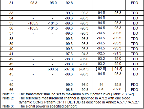
Read across a row rather than down a column. The steps between the bandwidths are the same in every band, and they are not arbitrary.

• Sensitivity gets worse as the channel widens : band 1 reads -99.3, -96.3, -94.5 and -93.3 dBm at 5, 10, 15 and 20 MHz.
• Those steps are the noise bandwidth and nothing else : doubling from 5 to 10 MHz costs exactly 3.0 dB. The half step to 15 MHz costs 1.8 dB and the last one costs 1.2 dB.
• The same three steps appear in other bands : band 2 runs -97.3, -94.3, -92.5 and -91.3. That is the same 3.0, 1.8 and 1.2 dB.
• A dash means the bandwidth is not defined in that band : band 1 has no 1.4 MHz or 3 MHz entry at all.
• Square brackets mean the value is not yet agreed : band 44 carries its whole row in brackets.
• Note 1 is the one that explains the test above : the transmitter shall be set to maximum output power. So the receiver is measured while the UE is transmitting as hard as it can.
• Note 3 places the level per port : the signal power is specified per port. So a two antenna UE receives that level on each.

NOTE : P_REFSENS is the reference that is used to derive the Reference Ior. Based on 36.521-1 cl.3.2, the reference Ior can be derived by taking P_REFSENSE * (N_SC_RB * N_RB * df) where df = subcarrier spacing. Roughly speaking this is the total channel power received at UE Rx antenna. If we allocate full RB, Ior can be almost same as P_REFSENSE.

Step 8 : Measure the average throughput.

Thinking over a cup of coffee

The two pictures below are here as questions rather than as answers. Each one holds a result that looks wrong until you work out which part of the transmitter produced it. Both repay a minute of thought before the bullets underneath them.

The first one sweeps the transmit power across four plots and leaves everything else alone. The allocation is the full 100 resource blocks in all four.

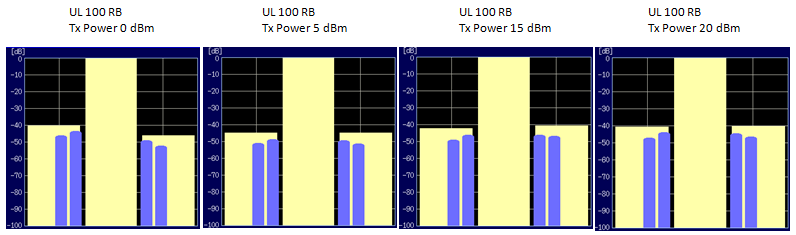
Twenty dB of transmit power across these four plots, and the bars that matter barely move. That is the answer hiding in the picture.

• All four plots are the same allocation : UL 100 RB. That is the full 20 MHz, at 0, 5, 15 and 20 dBm transmit power.
• The wide block in the middle is the wanted channel : it is the 0 dB reference. The vertical axis runs down to -100 dB from it.
• Two blue bars sit either side : the first and second adjacent channels, at roughly -42 to -50 dB in every one of the four plots.
• Those bars hardly move across 20 dB of power : that is the point of the picture. It is what makes ACLR a ratio rather than a level.
• A ratio is what the amplifier holds until it is pushed : leakage and wanted power rise together while the amplifier stays linear, so their ratio stays put.
• The limit would be reached by compression, not by power alone : the picture stops at 20 dBm, and the interesting region is above it.

The second one moves the allocation instead of the power. Three plots, each across the same 100 resource blocks, with the transmission placed low, in the middle and high.

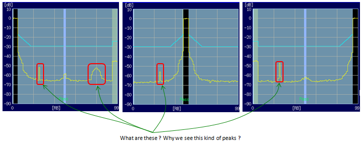
The question written under the picture is the author's. The answer is in the in-band emission drawing further up this page.

• The horizontal axis is resource blocks, not frequency : 0 to 99, which is the 100 blocks of a 20 MHz channel.
• The black band in each plot is the allocation : at the low end in the left plot and near the middle in the centre one. The right plot puts it at the high end.
• The red rectangles mark peaks that sit away from the allocation : the green note underneath asks what they are and why they appear.
• They move when the allocation moves : that alone rules out the instrument and the channel, because neither would follow the scheduler.
• The drawing higher up this page names them : Emission by Carrier Signal and Image created by Carrier Signal and Transmitted Signal. Those are the two unwanted features of a direct conversion transmitter.
• 36.101 treats them as two separate requirements : clause 6.5.2.2 is Carrier leakage and clause 6.5.2.3 is In-band emissions.
• This is why the IBE limit is written per resource block : a limit fixed to one part of the channel would pass or fail on the scheduler's choice alone.

• One test is a ratio and the other is a position : ACLR barely notices the transmit power, and in-band emission barely notices anything else.
• A peak away from the allocation is usually the transmitter, not the channel : carrier leakage sits at one fixed place and the image sits opposite the wanted signal.
• Both pictures argue for sweeping the right variable : power for one and allocation for the other. That is exactly what the test configuration tables in this page do.

Reference

The documents below are the ones this page works from. The test numbering and the test configuration tables come from the first two, and the connection diagrams from the third. Only the clause list of the fourth could be read here.

• 36.521-1 : 3GPP - E-UTRA; User Equipment (UE) conformance specification; Radio transmission and reception; Part 1: Conformance testing. The source of the chapter 6 and chapter 7 test numbering, and of Tables 6.2.2.4.1-1, 6.2.3.4.1-1, 7.3.4.1-1, 7.3.5-1, C.0-1 and A.2.2.2.1-1.
• 36.521-3 : 3GPP - E-UTRA; User Equipment (UE) conformance specification; Radio transmission and reception; Part 3: Radio Resource Management (RRM) conformance testing. The source of the RRM chapter list in the section of the same name.
• 36.508 : 3GPP - Common test environments for User Equipment (UE) conformance testing. Annex A holds the connection diagrams reproduced on this page. Clauses 4.1 and 4.3.1 hold the test environments and frequency ranges the configuration tables point at.
• 36.101 : 3GPP - E-UTRA; User Equipment (UE) radio transmission and reception, v20.0.0. Clause 6.5.2 holds the transmit modulation quality requirements, with Carrier leakage at 6.5.2.2 and In-band emissions at 6.5.2.3.