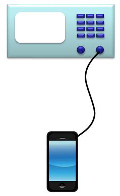
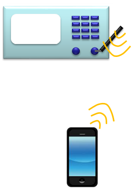
OTA stands for Over The Air. In order to perform test a device with any test equipment, you need a way of connecting the device to the test equipment. OTA is a kind of method connecting a device to a test equipment. There are roughly two kinds of connection method as shown below. One is Conductive and the other one is Radiative (or OTA). Simply put, OTA is a connection method via a pair of antenna (Transmiting antenna and Recieving Antenna).

The table shown below sets the two connection methods side by side. The left column is Conductive, where a cable carries the signal between the instrument and the device. The right column is Radiative, where a pair of antennas carries it and no cable joins the two.

Actually OTA is a very complicated topic. There are many different aspect to think of. I will try to cover as many different perspective as possible as I learn and experience more.

• Types of OTA Setups
• Why OTA ?
• UE Placement in Test Setup (Antenna Distance between UE and Test equipment)
• Why testing in Far Field ?
• Why Antenna Dimension is so important ?
• Handling Known-D situation and Unknown-D situation (Whitebox vs Blackbox Approach)
• Emulating a Black Box with Not-Too Big Chamber - CATR
• SS_MPAC(Simplified Sectorized MultiProbe Anechoic Chamber)
• Quiet Zone
• Reference

Types of OTA Setups

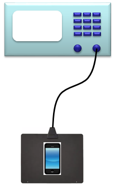
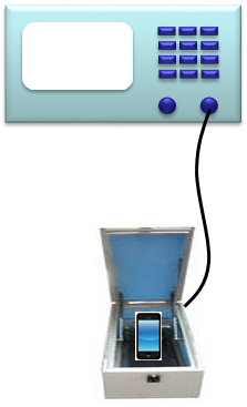
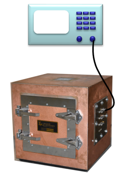
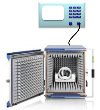
When we say Radiative testing, it usually refers to various different types of configurations as shown below. These are just a few typical examples that you may see most often, but these are not all. There are so many different variations of Radiative Test Setups. Even though the terms OTA Test and Radiative Test can be used interchangeably, when we say OTA test without any specific details, we normaly think of the configuration like (C) or (D) shown below. As shown below, it is test in a chamber lined with absorbers (this kind of chamber is called Anechoic chamber. Anechoic means 'No Echo'. 'No Echo' in this case mean 'No reflection from any object in the box).

Why OTA ?

Even in conventional technologies (e.g, UMTS, LTE), sometimes we performed OTA measurement especially for TRP or TIS measurement. However, in 5G/NR we are talking about OTA with almost every test, even with protocol test. Why OTA has become such a big issue in 5G/NR ? In NR, there are roughly two separated spectrum that are specified in 3GPP specification. One is FR1 (sub 6 Ghz) and the other is FR2(mmWave). In FR1, we may continue to go with the conductive testing as we do with 2G/3G/4G technology. However, in FR2 it is highly likely that we are forced to go with OTA. Why ?

We can think of several reasons for this and with a few different aspect.

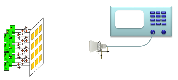
• Complexity : In FR2, it is almost sure that we will use some type of array antenna (called Massive MIMO). It means you will have a lot of antenna on the device. If you want to go with conductive testing, the connection would goes like (B) shown below, whereas you can do test as in (A) if you go with OTA. Then, it would be obvious on why we want to go with (A). NOTE : If you want to ask why we need to use an Antenna Array, Motivation of Massive MIMO page would give you some insight.
• Not Enough Space : Let's assume that you have enough reason to go with OTA despite the complexity of cable connection, you would still face another serious issue. Even though many of the antenna element (e.g, 16, 32, 64 etc) in your antenna array, the whole size of the antenna module would not be large enough at mmWave frequencies to accommodate all the cable connectors.  
• Cost : Now let's assume that you have really, really serious reason to go with conductive (like B) despite all the complexity and space issue. Even in this situation, there is other problem with conductive test. In most of conventional test, you might have used low cost SMA connectors and cables. However, you would not get the accurate measurement with SMA type of connector / cables in mmWave. You would need K connector or even more special connectors and cables (e.g, V connectors) if the freuqency goes even higher. These types of special connectors and cables cost much higher than those SMA types. If we need to use very high frequencies (like over 60 Ghz) in the future, you may need to spend in just for connectors and cables almost as much money as a low cost equipment price.
• Physical Nature of the Measurement : Even when you overcome all the issues described above, there is certain types of measurement that requires OTA because of the nature of the measurement itself. For example, if you want to detect the direction of the beam formed by the antenna array, you must rely on OTA measurement. You may say that you can still do this by conductive test. Theoretically, you can bring all the signals from each of antenna element path down to baseband and figure out beam direction (and other nature of the beam) by baseband processing. Of course, theoretically this is possible. But I am 100% sure that you want to avoid doing this if there is a relatively easy way like OTA test.

The table shown below contrasts the two ways of reaching an array. (A) radiates to a single horn antenna connected to the instrument, and (B) runs one cable per element, which is the difference the four reasons above are really about.

UE Placement in Test Setup (Antenna Distance between UE and Test equipment)

In order to get a repeatble, reliable and stable measurement result, it is very important to place the AUT(Antenna Under Test) and the measurement antenna in proper position. In this section, I will explain on how to determine the proper antenna position and theoretical background on why the specific posiiton should be used.

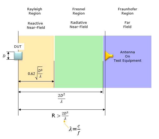
Minimum far-field distance R for a traditional far field anechoic chamber are determined by the formula a shown below (Based on R5-180013).

The figure shown below divides the space in front of an antenna into three named regions and gives the boundary between each pair. The DUT and its dimension D sit at the left edge, and the antenna on the test equipment sits out in the region on the right.

< Figure 1 : Antenna Field Region >

The near/far field boundary for different antenna sizes and frequencies is shown in the table below. This table is based on  R5-180013 (Ref [1]) - Table 2.2.1: Near field/far field boundary for different frequencies and antenna sizes for a traditional far field anechoic chamber

The table shown below turns that boundary formula into numbers. It sweeps the antenna dimension D from 5 cm to 30 cm at two frequencies, 28 GHz and 100 GHz. Each row gives the resulting boundary distance and the path loss at that distance.

< Table 1 - Near/Far Boundary distance with D and Frequency >

NOTE : From this is the optional reading. I've looked into the equation a little bit deeply just out of curiosity. If may skip this part if you are not interested. I tried to investigate on how the near / far boundaries changes as frequency changes.

As shown below, the span of Radiative Near Field (the gap between the end of Reactive Near Field and the Start of Far Field) gets drastically increases as frequency increases where as Reactive Near Field distance relatively slowly increases). Also, comparing the following two plots, you would notice that the Far Field distance gets drastically larger as D increases.

The figure shown below plots both boundary distances against frequency for a fixed antenna dimension of 5 cm. The upper trace is the far field boundary and the lower one is the reactive near field boundary, so the gap between them is the radiative near field.

< Figure 2 - Field Boundary change with frequencies at D = 5 cm >

The figure shown below repeats that plot with the antenna dimension doubled to 10 cm. The axes are unchanged, so the two can be compared directly, and the far field trace now reaches about four times as far at the same frequency.

< Figure 3 - Field Boundary change with frequencies at D = 10 cm >

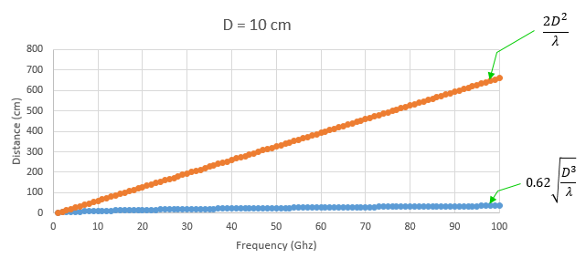
Now you may have an interesting question. According to the plots shown above, the distance between DUT antenna and equipment antenna should increase as frequency increases. That is, the size of Anechoic chamber should increases as frequency increases ? Isn't it counter intuitive to you ? Our common sense (our RF intuition) says the size of frequency dependent object tend to decrease as frequency increases.

How do we handle this conflict with our intuition and the plots show above ?

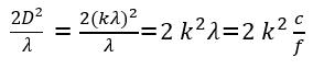
The solution lies in the fact that D is not a constant in realilty. In case of plots shown above, D has a fixed value regardless of frequency. But when we design an antenna, we usually decide D value(Antenna Aperture size) in terms wavelenth as shown below. Here, k is just a constant like 0.5, 1, 2 etc.

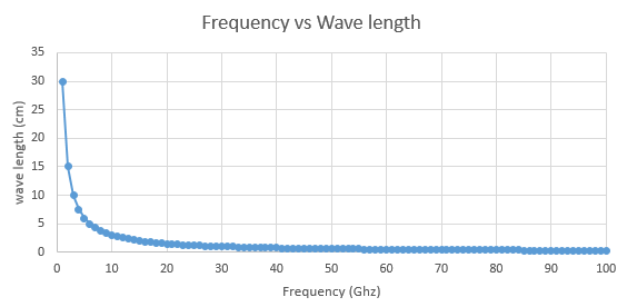
If you plot on how wavelength (lamda) changes as frequency increases, you will get a plot as shown below. You will notice that the wavelength decrease dtrastically.

The figure shown below plots wavelength against frequency, and it is the piece that explains the two plots above. Wavelength falls from about 30 cm at the left edge to under 1 cm above 30 GHz, and the far field formula divides by that quantity.

< Figure 4 - Wavelength vs Freuqnecy >

If you rewrite Far Field distance equation, it becomes as shown below. In this equation, you will notice that the Far Field distance decreases as frequency increases.  (NOTE : if you want to try calculate in real value, take f as 'frequency in Hz' and c as 'the speed of light in m', k is just a constant without any unit).

Why testing in Far Field ?

Probably by now, you may have a question 'Why do we need to test in Far Field ?'.  It would not be easy to get a direct answer to this question. So let me change the question a little bit. Why we do not test in Near field ?

The simple answer to this question is that the measurement result in this region tend to be unpredictable and subject to change with small changes in the environment surrounding the antenna(e.g, electrical circuit feeding the antenna) and location changes. On the contrary, the field pattern in Far field is more stable and predictable and less senstive to small surrounding components.

For those who are interested in further details, let's look a little bit further details on the characteristics in each of the region. You may investigate even further on your own. Try googling the keywords like 'Near and Far Field', 'Field Region around Antenna' etc.

Reactive Near Filed : This is the area that is very close to the antenna. The relationship between E and H field in this region is very unpredictable (It is unpredictable not because this property goes against a physical theory, but because the physical property is so complicated). For example, at one point you would see E field dominates and at another point right besides the previous point H field dominates.  Also radiated energy would influence back and forth with surrounding electrical component like antenna control circuit. For example, some portions of radiated energy gets absorbed and stored in surrounding component at some point of time and the stored energy gets radiated back into the space at other point of time and influence radiation pattern.

Radiative near field (Fresnel region) : In this region, the distance from the antenna is not so close to be influenced by reative electrical components as described above and the E and H field relationship is much more predictable comparing to Reactive Near Field. However, the E and H field relationship is still pretty complex and there are high possibilities where some physical object that may affect the radiation pattern in this area. For example, some metal object like steel beam holding up the antenna module can act as a kind of antenna or reflector. So this kind of object can influence on the radiation pattern of the AUT(Antenna Under Test).

FAR field (Fraunhofer region): In this region, the angular field distribution is essentially independent of the distance from the antenna and the radiation pattern can be approximated with spherical wave-fronts. Since any recieving point in the region are very far from the antenna, the transmitter size and shape are not important anymore and it can be approximated as a point source. The electric and magnetic fields are in phase, perpendicular to each other and perpendicular also to the direction of propagation. In this region, you can safely assume that the wave front going through the recieving antenna is planner (i.e, all the incoming rays are in parallel to each other). Putting it simple, this is the idea region in which most of measurement can be done easily and reliably.

Why Antenna Dimension is so important ?

As mentioned above, in order to achieve the stable measurement result it is important to put the distance between DUT antenna and the equipment antenna to be greater than the Far Field Boundary. As shound in [Figure 1], the Far Field boundary starts from the following distance.

As you notice from this expression, the distance is proportional to D squared (D represents antenna dimension). That is, the distance changes drastically with even a small changes in D. To give you more intuitive understanding, I plotted this equation in a graph as shown in left. The path loss at the boundary also increases as the D increases as shown in right.

The figure shown below holds the frequency at 28 GHz and sweeps the antenna dimension instead. The left plot is the far field boundary distance and the right one is the path loss at that distance. Both costs of a larger antenna therefore appear side by side.

< Figure 5 - Far Field Distance and Path Loss with D >

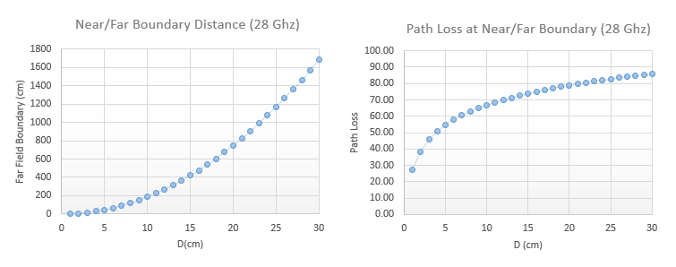
In case that you want to get the exact quantitative data, I put a table as shown below. The two graphs shown above are plotted from this table.

The table shown below is the numeric form of those two plots. It steps D from 1 cm to 30 cm at 28 GHz. The square law in the boundary column and the slower rise in the path loss column can therefore be read row by row.

< Table 2 - D influencing on Far Field Distance and Path Loss >

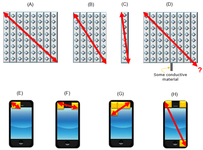
What this implies is that you need to know the exact antenna dimension in order to get the accurate measurement. However, it is not always easy to correctly define the antenna dimension. Antenna Dimension D is defined as the maximum distance across the whole antenna module. The Red Arrow in [Figure 6] indicates D. As you see, it would be straightforward to define D in case of (A), (B), (C) and (E). However, in case of (D), defining the dimension would not be so easy. In (D), the physical dimension is same as (A), but you see some conductive material around the antenna module influence the radiation pattern of the antenna module. This may influence the effective dimension of the antenna and it would be very difficult to accurately estimate the effective dimension. Also there would be some possibilities where UE makers distribute the antenna modules accross several different locations inside of the UE as shown in (F), (G) and (H). Of course, the shape and location of Antenna modules within a UE would be more diverse and complicated than the ones shown here.

The figure shown below is why defining D is not straightforward. It draws eight cases lettered A to H, and the red arrow in each one marks the dimension the far field formula needs. The first four are bare arrays and the last four are antennas inside a phone.

< Figure 6 - Antenna Dimensions for various configuration >

There is another reason why defining D gets difficult. It would get more difficult for UE case. In order to correctly define D, you need to have all the detailed information of the antenna structure and positions in UE. But in many cases these information is treated as a highly confidential information by most of UE manufacturer. So when you are given a UE (especially a commercialized UE), it is almost impossible to get the exact estimate for D (Dimension).

Now we are facing a very tricky situation. How can we guarantee the accurate measurement when we are not given the detailed information on Antenna dimension ?

This is what I will talk about next section.

Handling Known-D situation and Unknown-D situation (Whitebox vs Blackbox Approach)

Before getting into specific cases, let's think of the meaning of a few basic words - Whitebox and Blackbox. Whitebox refer to a box we can directly look into the box and clearly knows what is inside of the box. It means all the information about the box is known to ux. Blackbox refer to a box we have no direct visibility to the inside of the box. The only way that we can figure out the contents of the box is via indirect observation like shaking the box and listen to the sound or lifting up and estimate the weight etc. Of course, this is not the formal definition of Whitebox and Blackbox in OTA, but the basic idea applies to the formal definition as described in R4-1708553 (Ref [4]).

For the Black box approach, the exact antenna locations/centre-of-Radiation-Reference-Point (CORRP) do not need to be known.

• The UE is positioned with a common reference point similar to existing SISO OTA test cases
• Execution of test cases have relatively low complexity (repositioning to CORRP will not be necessary)
• An MU element for Offset DUT phase centre from centre of QZ(Quiet Zone) will need to be added for the DUT stage of the MU budget which depends on size of QZ, and range length

For the White box approach, the exact antenna locations/centre-of-Radiation-Reference-Point (CORRP)  need to be known, likely via a manufacturer declaration.

• The CORRP for the active antenna array needs to be aligned with the centre of the quiet zone which likely yields complex execution of test cases
• An MU element for Offset DUT phase centre from centre of QZ(Quiet Zone) will not need to be added for the DUT stage but a MU element for UE re-positioning needs to be added

Now you may ask 'Why we are talking about whitebox / blackbox concept here ?' and 'how are they related to handling D(Antenna Dimension) ?'.  Let's think of a situation where we have the detailed information on D and a situation where we don't have exact information on D.

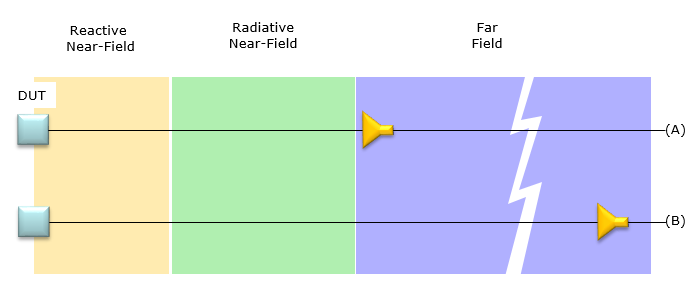
Let's assume that we have all the detailed information about D. It means the Antenna module under test is a kind of whitebox. In this case, we can calculate the exact location of Near / Far boundary. Then we can get relatively accurate measurement with the minimum distance between DUT and Measurement Antenna(Probe) and still meeting the Far field criteria as in (A) of [Figure 7]. It means that we can meet the Far Field condition with minimum size of Anechoic chamber. In turn, it means we can get the accurate measurement with minimized cost on Anechoic chamber.

Now let's think of a situation where we don't have accurate information on D. How we can estimate the exact location of Near/Far boundary (i.e, Starting point of Far Field) ?  The answer is 'There is no way to do it'. Then how we can guarantee that the antenna is in Far Field ? The simplest way is to place the receving antenna at a position which is very far away from the DUT so that you can assume that it is in Far field regardless of the size of antenna as in (B) of Figure 7. Of course there should be a certain limitation of Antenna size you assume. You would not assume that the antenna size is 20 cm when you have a mobile phone with the size of 10 cm.

The figure shown below places the measurement antenna at two different distances against the same three field regions. Case (A) is the whitebox distance and case (B) is the blackbox distance. The break drawn across the far field marks how much further out (B) has to sit.

< Figure 7 : Possible Antenna Location in Whitebox and Blackbox condition >

Wrapping up,

we may say if we can get the detailed information on Antenna dimension and exact antenna location on DUT (e.g, Mobile phone), it would be better to use Whitebox approach, since we can do the measurement with smaller chamber and at relatively low cost. This can be a good option at the development stage in which these informations tend to be open.

If the detailed information on Antenna dimesion and locations on Mobile phone, Blackbox approach will be the better option. Since most of the mobile phone manufacturer would be very reluctant to open the detailed information on antenna on their commercialized device, the blackbox approach may be the only option for the commercialized device. However, as mentioned above, we would need very large chamber to apply the blackbox approach which would cause cost and space issue. To mitigate this problem, an alternative concept were proposed and this alternative will be explained in next section.

NOTE : Regarding the adoption of Whitebox approach or Blackbox approach, Ref [3] states as follows :

For conformance testing, 3GPP has decided that only the black box approach can be used. This is due to the requirements for white box testing not being accepted by UE vendors who preferred not to declare the antenna structure.

Emulating a Black Box with Not-Too Big Chamber - CATR

As mentioned above, it is likely for only blackbox approach to be accepted as a test method for commercialized device since UE manufacturer does not like to disclose the detailed antenna information, but blackbox approach tend to require huge chamber (i.e, large distance between the transmitter and reciever antenna). To reduce the problem of the chamber size issue an alternative concept called CATR(Compact Antenna Test Range). The overall concept is described in TR 37.842 as shown below.

The figure shown below is the CATR arrangement as TR 37.842 draws it. The reflector on the right is the part that does the work. Everything else is an ordinary anechoic chamber with a positioner, a feed antenna, and the instruments outside the chamber wall.

< TR 37.842 - Figure 10.3.1.1.3.1-1: CATR measurement system setup for EIRP >

Figure 8. The long dimension of the chamber is not the measurement distance. The reflector turns the feed antenna into a source at infinity. The DUT therefore sees a plane wave inside a box far shorter than the far field formula demands.

• The DUT sits on a positioner at the upper left, and the chamber walls are lined with absorber on every side.
• The range antenna reflector is the curved surface on the right, and the blue lines between it and the DUT are drawn parallel.
• The feed antenna sits below the reflector, and the lines between the feed and the reflector fan out rather than running parallel.
• A coordinate triad marks z upward and x to the right, with y into the page.
• The positioner controller, a PM/SG and a PC sit outside the chamber and are wired to the positioner and the feed.

As shown above,  you will see the signal from the transmitter antenna bounces (reflects) from a specially designed reflector and then reaches to the receiver antenna. This would take an effect of folding up a long linear distance into a small space, which result in reducing the size of the chamber. In addition, by designining the reflector in a specific form, you can make all the parallel rays from DUT reaches to Feed antenna(measurement antenna). And, also you can make the rays from the feed antenna reaches DUT as parallel rays. Actually the basic principle is similar to what you learned in high school physics about Ray diagram of Parabolic mirror. Try googleing 'Parabolic Mirror Ray Diagram' or 'Parabolic Mirror Ray Tracing' etc.

CATR is one of three answers 38.810 gives to the distance problem, and naming the other two puts it in context. Clause 5.2.1 defines the Direct Far Field method, which places the measurement antenna beyond the far field boundary and accepts the chamber length that requires. Clause 5.2.3 defines Indirect Far Field method 1, and 38.810 says that method creates the far field environment using a transformation with a parabolic reflector. That method is CATR.

Clause 5.2.4 defines the third answer, the Near Field to Far Field transform. That method measures inside the near field and computes the far field metrics from what it captured, so it trades chamber size for processing rather than for optics. 38.810 also defines a simplified Direct Far Field setup in clause 5.2.2, for centre of beam measurements only.

• CATR replaces distance with optics : the reflector collimates the feed, so the DUT sees a plane wave without the chamber being far field long.
• It is the indirect method, not a shortcut : 38.810 files CATR under Indirect Far Field method 1, and the far field condition is met rather than waived.
• Three methods exist, not one : Direct Far Field needs chamber length, CATR needs reflector quality, and the Near Field to Far Field transform needs computation.
• The reflector becomes the error source : once the chamber is short, the accuracy of the plane wave depends on the reflector surface rather than on the distance.

SS-MPAC (Simplified Sectorized MultiProbe Anechoic Chamber)

The concept of SS MPAC is to use multiple probes around UE as illulstrated below to emulate more realistic radio channel condition. Every method described so far measures a device against one probe at a time, which answers how well the device performs along one direction. A real channel arrives from many directions at once, and that is what this setup is built to address.

The figure shown below is the probe geometry from R4-1706669. It is a three dimensional plot rather than a chamber drawing, so the axes are marked in metres and the small circles are probe positions rather than physical hardware.

< R4-1706669 : Figure 2. Installed probes in the sector and UE >

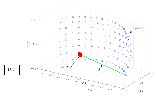
Figure 9. The probes cover a sector rather than a sphere, and that is what the word Simplified in the name refers to. A full sphere of probes would measure more and cost far more.

• The DUT array is the red block near the origin, labelled DUT array, and a separate box on the left is labelled UE.
• The small blue circles are the probes, and they are arranged on a curved surface rather than on a flat plane.
• The probes occupy one sector of that surface, so they surround the DUT on one side only.
• The green line labelled R runs from the DUT array out to one probe, and it is the radius of the probe surface.
• All three axes are marked in metres and run from -1 to 1, so the whole arrangement is about two metres across.

The major motivation of SS MPAC is well described in R4-1706669 as follows :

1. Realtime system performance assessment, i.e. while communicating

2. Capable of emulating realistic radio channels, meaning with realistic angular distributions of waves, either irradiating EU or being radiated by it

3. Up and downlink performance, or reception and response in multinode configurations

The three motivations above are worth reading against the earlier sections of this page. A CATR or a Direct Far Field chamber measures a radiated quantity with the device idle or on a fixed beam. The first motivation asks for measurement while the device is communicating, which no single probe setup provides. The second asks for a channel with a realistic angular distribution, and a single probe has exactly one angle.

• Sectorized means a partial sphere : the probes cover one sector, which is the compromise that separates this setup from a full multi-probe chamber.
• The target is beam management, not just power : several probes at different angles let the device choose a beam, and that choice is what the measurement observes.
• It is an RRM and demodulation method : R4-1706669 proposes it for those tests rather than for the RF power measurements the earlier setups cover.

Quiet Zone

According to Ref [9], Quiet Zone is the volume in any chamber in which a DUT is illuminated with nearly uniform amplitude and phase. Typical quiet zone specifications are 10 degrees of phase variation, 0.5 dB of amplitude ripple, and 1 dB of amplitude taper, which is the roll-off toward the edges of the quiet zone

The quiet zone is where every other number on this page is actually claimed. A far field distance, a path loss figure and a beam measurement all assume the device sits somewhere the illuminating wave is uniform. The quiet zone is the name for that somewhere, and its size sets the largest device the chamber can measure at the stated uncertainty.

38.810 ties the definition to the mechanics of the setup. In a Direct Far Field arrangement the centre of the quiet zone sits at the centre of the rotational axes, of the DUT and of the measurement antenna together. That centre is then taken as the reference point for defining measurement uncertainty. Move the device away from it and the uncertainty budget no longer describes the measurement being made.

Quiet zone quality is measured rather than assumed. 38.810 lists it as a measurement uncertainty contributor in the annex for every setup it defines. 38.827 devotes Annex D to the characterisation procedure, with separate procedures for FR1 and FR2.

• The quiet zone bounds the device size : a DUT larger than the zone is partly outside the uniform field, so the uncertainty budget no longer describes it.
• Its centre is a mechanical point : 38.810 puts it at the centre of the rotational axes, which is why positioning repeatability matters as much as chamber size.
• Quality is a measured quantity : 38.827 Annex D gives the characterisation procedure, and 38.810 carries quiet zone quality as an uncertainty term in every setup annex.

Reference

[1] 3GPP TSG-RAN WG5 Adhoc Meeting#1 - R5-180013 : Signalling NR Testcases - OTA chamber requirements

[2] Near and far field (Wikipedia)

[3] Keysight Technologies - OTA Test for Millimeter-Wave 5G NR Devices and Systems (White Paper)

[4] 3GPP TSG-RAN WG4 Meeting #84 - R4-1708553 : Far field definition and proposal for alternate RF baseline with deterministic antenna array positioning

[5] 3GPP TSG RAN WG4 Meeting NR#2 - R4-1706617 : Center of Radiation Reference Point Reference Definition for OTA Measurements of Phased Array Beamforming Patterns

[6] 3GPP TR 37.842 V13.2.0 (2017-03) - Radio Frequency (RF) requirement background for Active Antenna System (AAS) Base Station (BS)(Release 13)

[7] 3GPP TSG-RAN WG4 Meeting NR AH#2 - R4-1706669 : SS MPAC for RRM/Demod  

[8] TR 37.977 - Verification of radiated multi-antenna reception performance of User Equipment (UE)  

[9] OTA Test for Millimeter-Wave 5G NR Devices and Systems (Keysight Whitepaper) 

[10] 3GPP TR 38.827 - Study on radiated metrics and test methodoloty for the verification of multi-antenna reception performance of NR User Equipment (UE).