|
4G/LTE - Basic Procedures |
||
|
LTE PHY DSP(Digital Signal Processing)
This note is based on my recent trial to decode and analyze LTE PHY signal. This is mainly to refresh my memory about the analysis process and method, but I hope it will be of help others as well. It is not the program that process the signal real time. It was a script that I wrote in Python that process the baseband I/Q data captured from Amarisoft eNB.
NOTE : The baseband signal data (I/Q) data is captured with following condition.
Followings are the list of procedure that I went through.
The first step to decode LTE PHY signal is to detect PSS and extract additional helper information. Personally, I think this would the most important step for LTE PHY signal processing because without this process you may not be able to decode any other signal. This process involves multiple steps and each of those step can be a topic for separate note. For the details of nature of PSS itself and detailed algorithm to detect PSS, check out this note. In this note, I would just give you a big picture about result of PSS detection.
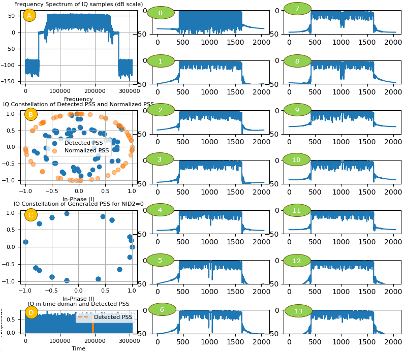
Following is a series of plots from my script with the detection of PSS.
[D] represents the absolute values of I/Q data. This is the plot of raw (unprocessed) data. The only process part on the plot is the part shown in orange color. It is the part on which the detected PSS is overlaid. [A] is also a plot of non-processed data like [D]. The difference between [A] and [D] is difference between Time domain representation([D]) and Frequency Domain representation([A]) [B] is represent the detected signal (I/Q data) for PSS. The blue dots indicates the detected PSS as it is. Orange dots indicates the detected PSS projected onto the circle of radius 1. Since the blue dots does not give obvious visual correlation with the ideal PSS signal (a Zadoff sequence), I wanted to project it onto the circle like Zadoff sequence. [C] is the ideal data that corresponds to the detected PSS data. It is the sequence generated by the script based on 3GPP spec and N_ID_2 (PSS sequence number) found during the PSS detection process. [0]~[13] are the frequency domain plot for each OFDM symbol within the subframe where the PSS was found. Once PSS is found, we can figure out exact subframe and slot boundary of the subframe because PSS is always located in the same place (i.e, symbol 6 (7th OFDM symbol) in the subframe). With this fact, we can slice out each of OFDM data with exact start and end point. I cut out each OFDM symbols from the I/Q data and plot them in Frequency domain in dB scale.
One of the important information we can get from PSS detection is frequency error (frequency offset) which can be used to adjust (correct) frequency error of other signals (e.g, correcting frequency error of SSS). Frequency offset can be calculated / estimated as follows)
def frequency_offset_estimation(received_pss, expected_pss): phase_difference = np.angle(np.dot(received_pss, np.conj(expected_pss))) frequency_offset = phase_difference / (2 * np.pi * 62 / SampleRate) return frequency_offset
The details on each line of the code is as follows :
received_pss : an array of I/Q of the detected PSS in the form of complex number expected_pss : an array of I/Q of the PSS generated by 3GPP algorithm def frequency_offset_estimation(received_pss, expected_pss): # Calculate the phase difference between the received PSS and expected PSS # This is achieved by first taking the dot product of the received PSS and the conjugate of the expected PSS. # Then, the angle (or phase) of this product is taken. phase_difference = np.angle(np.dot(received_pss, np.conj(expected_pss)))
# Convert the phase difference into a frequency offset. # The frequency offset is calculated by dividing the phase difference by the product of: # 2 * pi (to convert from radians to cycles) # The number of subcarriers comprising PSS (which is 62 for LTE) # dividing by the sample rate to get the offset in Hz frequency_offset = phase_difference / (2 * np.pi * 62 / SampleRate)
# Return the estimated frequency offset return frequency_offset
NOTE : how phase_difference / (2 * np.pi * 62 / sample_rate) can indicate the frequency offset ? Phase and frequency are directly related: the change in phase over time is frequency. In mathematical form, it can be represented as dφ / dt = frequency. In the frequency offset estimation function, the phase difference is divided by the time duration of the symbol (which is the number of subcarriers divided by the sample rate), giving us the rate of change of phase, or frequency offset. In other words, the equation calculates the average change in phase per sample, which is then converted to Hz to represent the frequency offset. This frequency offset represents the difference in frequency between the received PSS and the expected PSS. This difference arises due to the Doppler effect or inaccuracies in the transmitter or receiver oscillators, among other reasons.
Once you get the proper frequency offset, you can compensate (correct) frequency error of other signals as follows.
signal : an array of I/Q data in the form of complex numbers. frequency_offset : frequency offset in Hz sample_rate : sample rate in samples / sec def correct_frequency_offset(signal, frequency_offset, sample_rate):
signal = np.array(signal, dtype=np.complex128) time = len(signal) / sample_rate correction = np.exp(-1j * 2 * np.pi * frequency_offset * time) corrected_signal = signal * correction
def correct_frequency_offset(signal, frequency_offset, sample_rate):
# Convert the input signal into a NumPy array of complex128 data type. # This ensures the signal can be processed with complex arithmetic operations required for frequency correction. signal = np.array(signal, dtype=np.complex128)
# Generate the time vector for the signal. # Instead of creating a time array that corresponds to each sample point, the code calculates the # total time duration of the signal by dividing its length by the sample rate. time = len(signal) / sample_rate
# Calculate the complex exponential correction term. # This term is used to shift the signal's frequency content. # The negative sign in '-1j' ensures that we're shifting the frequency in the opposite direction # of the detected offset, thereby correcting it. # Multiplying by '2 * np.pi' converts the frequency offset to radians. correction = np.exp(-1j * 2 * np.pi * frequency_offset * time)
# Apply the correction to the original signal by element-wise multiplication. # This shifts the frequency content of the signal, thereby correcting the frequency offset. corrected_signal = signal * correction
return corrected_signal
Once you detected PSS and SSS, you are almost ready to reconstruct the resource grid (i.e, OFDM symbol vs Subcarrier). But before you trying to reconstruct the resource grid there is one more step to do. The time domain I/Q data carries a certain length of Cyclic Prefix (CP) data. You need to remove this part first before you reconstruct the resource grid. The number of I/Q samples for CP varies depending on the LTE channel bandwidth as explained in this note.
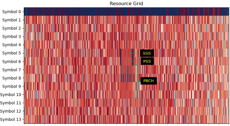
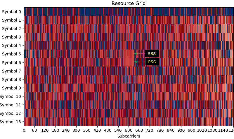
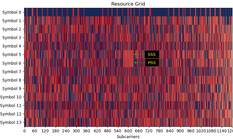
Once you have accuarate detection of timing and frequency boundary and removed CP properly, you can construct a LTE resource grid as follows. Once you have this kind of accurate resource grid, the retrieving and generating Physical layer data is something like reading and writing numbers in an Excel spreadsheet.
There is still one more step to do after you reconstructed the ResourceGrid after CP removal. It is the process of an subcarrier at the center of the resource grid.
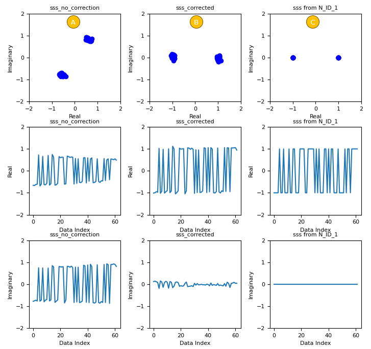
Once you able to construct an accurate resource grid as shown above, the first thing you need to do is to detect SSS(Secondary Synchronized Signal). This process is done as in the following step : i) Retrieve I/Q data from the resource elements for SSS from the Resource Grid ii) Compensate the retrieved SSS I/Q with frequency offset obtained by PSS detection procedure. iii) Generate all the possible SSS sequence that belong to the category for N_ID_2 (PSS sequence number) iv) Compare (correlate) each and every SSS sequence from step iii) with the SSS IQ data from step ii) and find the best pair. The SSS sequence index (N_ID_1) that gives the best correlation is the detected SSS. NOTE : The procedure for step iii) and iv) is explained in detail in this note.
Some highlights of SSS detection procedure are plotted below. (A) is the original IQ data retrieved from the resource grid(this corresponds to step i) mentioned above). (B) is the SSS data compensated by frequency offset (this corresponds to step ii) mentioned above). (C) is just one example of the generated SSS (this corresponds to step iii) mentioned above)
Now you have detected PSS and SSS. With the PSS sequence index (N_ID_2) and SSS sequence index (N_ID_1), you can calculated Physical cell ID (PCI) as explained in this note.
One of the most important thing in decoding the received signal would be to estimate channel characteristics and correctly equalize the received signal using the estimated channel characteristics. In LTE, we use cell specific reference signal (CRS) to estimate the channel characteristics (channel coefficient). To do this, we need to have the received CRS and the ideal/expected CRS. The first step required for retrieving the received CRS and expected CRS is PCI which is already obtained in previous step.
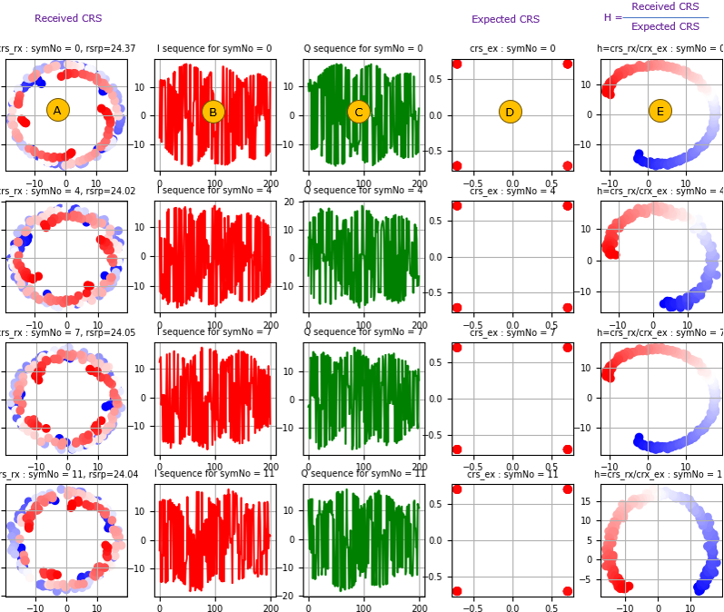
Once you have the accurate PCI, the process of estimating channel coefficient goes as follows (NOTE : this is for SISO case for simplicity). i) using the PCI, calculate the position of CRS. You can do this based on 3GPP specification explained in this note. ii) then retrieve the I/Q data(complex number) from the CRS position in the resource grid (let's store all these retrieved data to a variable crs_rx). iii) Now calculate the expected CRS for the specific PCI(let's store all these calculated data to a variable crs_ex). You can generate the expected CRS based on 3GPP specification explained in this note. iv) Once you have the received crs (crs_rx) and the expected crs (crs_ex), you can estimate the channel coefficient just takding "crs_rx divided by crs_ex". (NOTE : this is a simplified way assuming that it is SISO and noise level is very low.) For futher study on this process, check out this note and this slide. Following is an plots showing the result of some important steps described above.
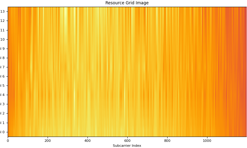
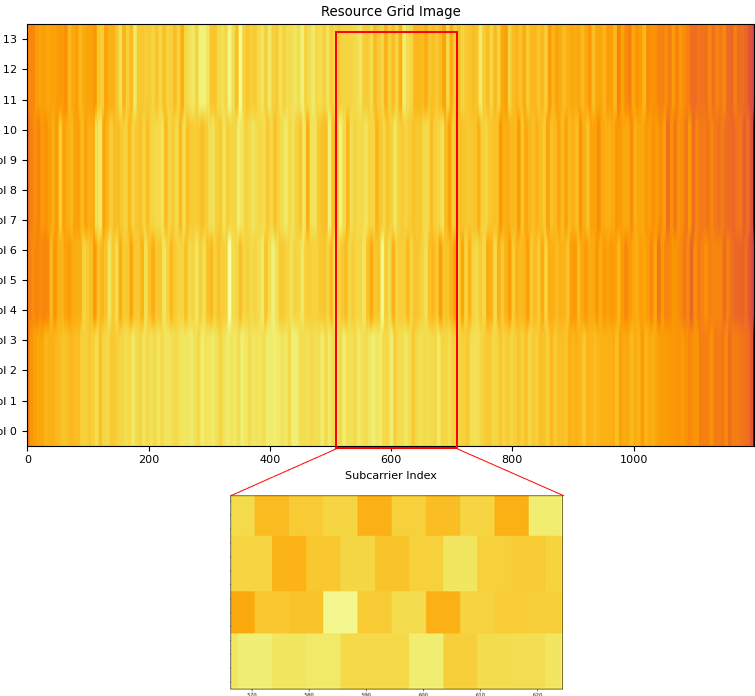
Now you got the channel coefficients for every resource elements where CRS is located. For the proper equalization for every resource elements in the resource grid, we need to figure out the channel coefficient for all other resource elements where there is no CRS. A common way to get the channel coefficient for every resource elements is interpolate the CRS channel coefficient in frequency and time domain and construct a resource grid filled out with the estimated (interpolated) channel coefficient. The plot for the channel coefficient resource grid (H resource grid) would be something like this.
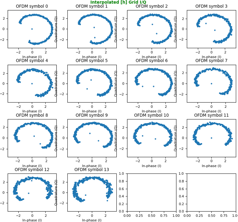
The heatmap shown above may look fancy but would not give you much concrete meaning. Proabably plotting constellation for each OFDM symbol would give you more meaning / intuition of the channel as shown below.
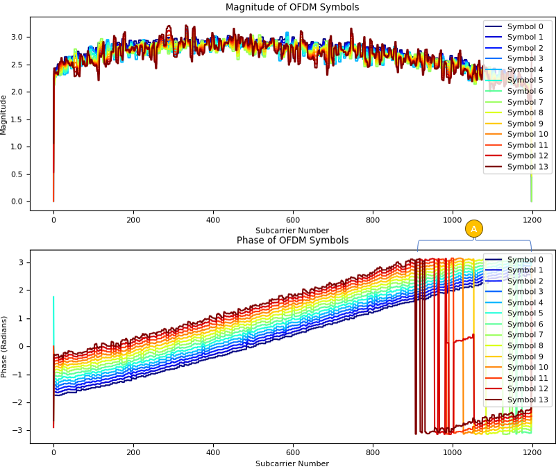
Just for a little bit different aspect (view point) of the channel coefficient for each resource elements, I plotted amplutude and phase plot for the H resource grid as follows. The smallest index on horizontal axis corresponds to the subcarrier at the lowest frequency.
Now let me show you how I got the full channel coefficient grid as shown above in step by step.
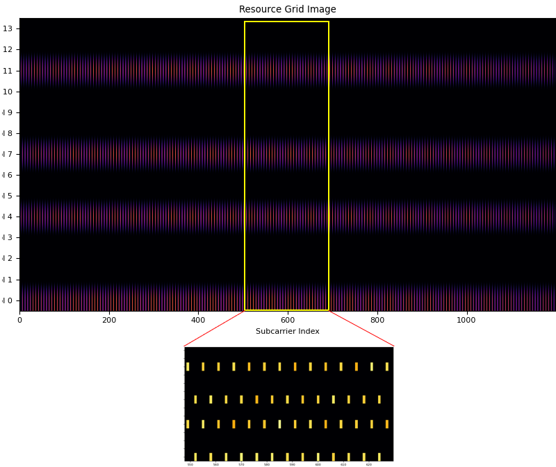
Step 1 : Populate H values into an empty resource grid
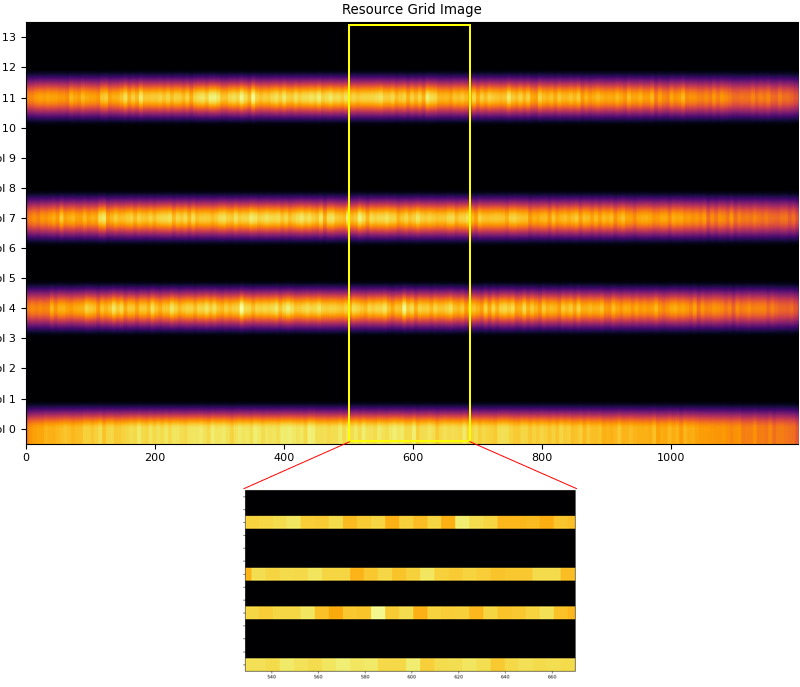
The first I did was to create an empty resource grid with same size as the data resource grid and the populate the H values for CRS at the proper CRS RE(Resource Element)s as shown below. You see that only CRS location has certain values (yellow / non-black) color and all other REs are empty (black)
Step 2 : Frequency Domain Interpolation
Now fill in the gaps only in frequency domain. You can do this by interpolating the values (complex value) along frequency domain. You may apply various ways of interpolation, but I did it just by moving average. The result of the frequency domain interpolation looks as follows.
Step 3 : Time Domain Interpolation
Now let's try to fill in the empty RE in time domain. Theoretically you can may use the same method as in frequency domain (moving average) or python package for the interpolation. But none of them work very good mainly because the number of points in time domain is too small. So I created my own interpolation function that can do the interpolation between only two end points. (NOTE : This is just for my own case, you may use different method of your own if you have any). Here is broken down procedure of what I did i) fill in symbol 1,2,3 by interpolating symbol 0 and 4 as end points ii) fill in symbol 5,6 by interpolating symbol 4 and 7 as end points iii) fill in symbol 8,9,10 by interpolating symbol 7 and 11 as end points iv) fill in symbol 12, 13 by extrapolating symbol 9,10,11 (You may do this by interpolating the symbol 11 and symbol 0 of next subframe, but I did the extrapolation because I processed only one subframe with no next subframe). Final result after all thse procedure, I get the resource grind as shown below.
With the resource grid filled with channel coefficient for every resource element, now we are ready with equalizing every symbols (every resource elements) and recovering constellation.
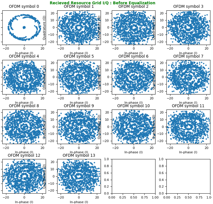
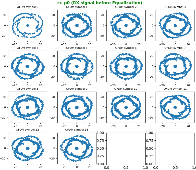
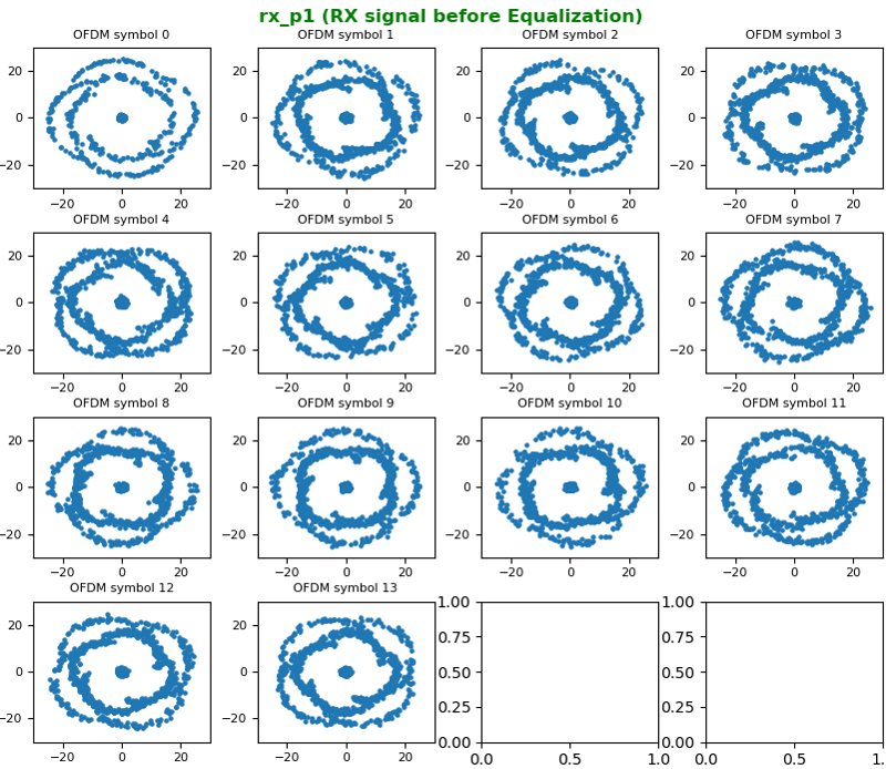
The constellation before correction (i.e, before Equalization), it looks as below.
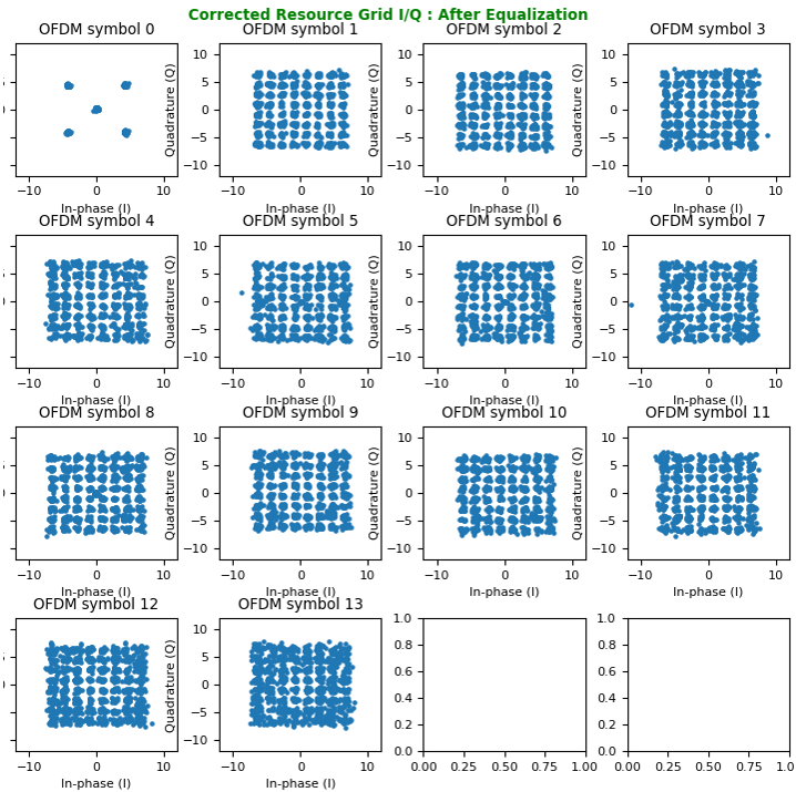
Now let's compensate (equalize) the constellation with the channel coefficient. With the equalization, we can get the nicely aligned constellation as follows. The basic idea behind the equalization can be represented by a simple math as follows : Corrected symbol (equalized symbol) = received symbol / channel coefficient
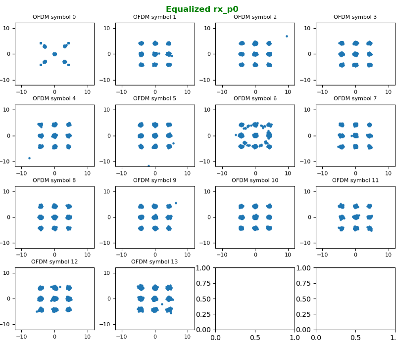
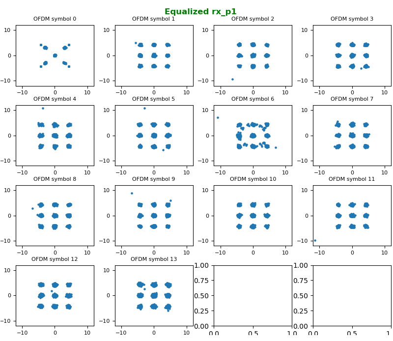
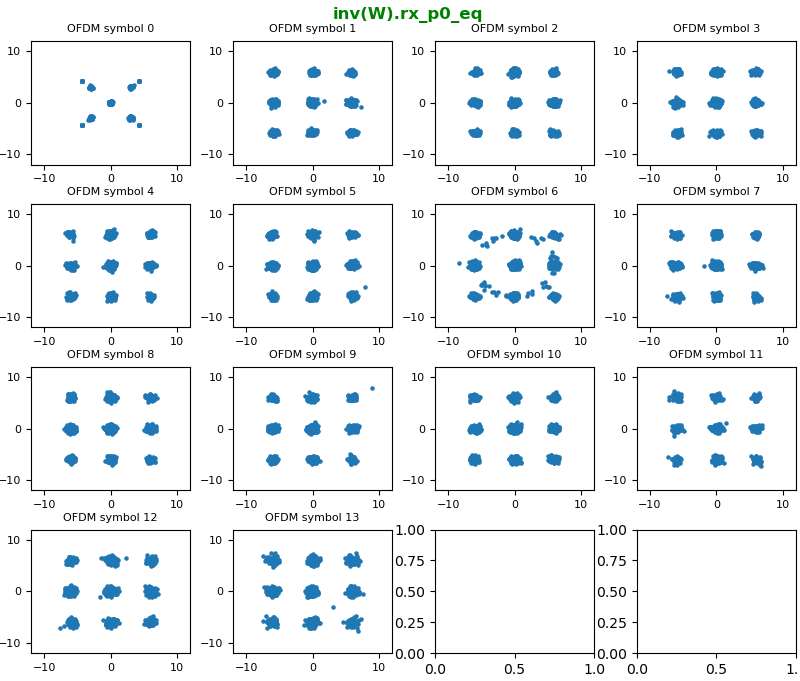
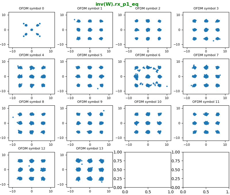
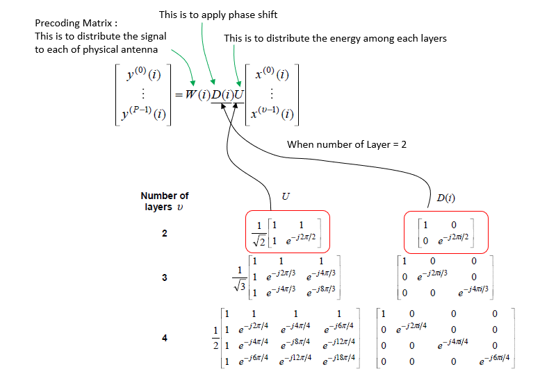
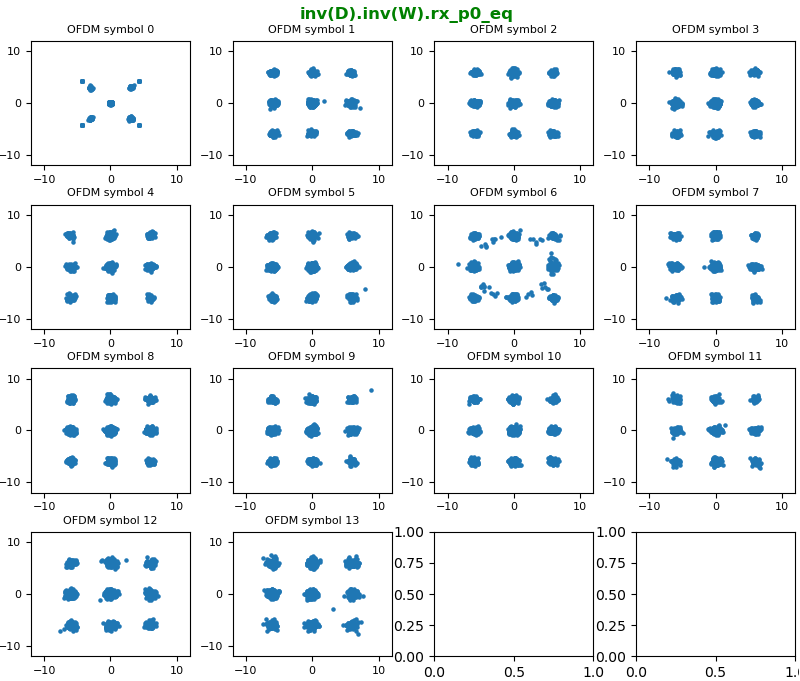
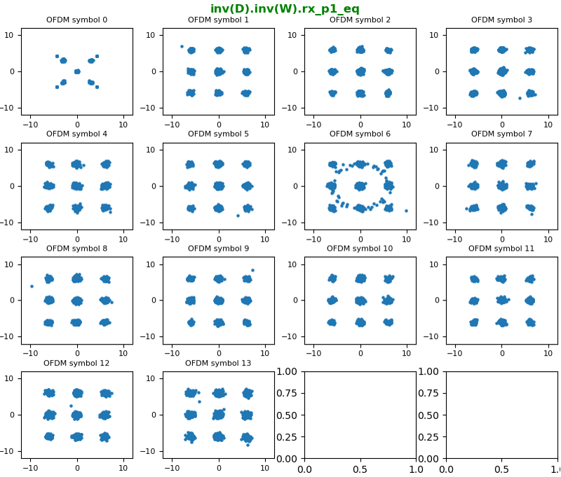
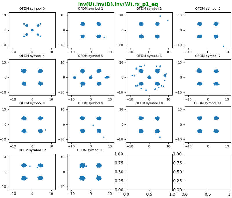
Processing 2x2 MIMO signal is basically similar to the processing of SISO, but it just a little bit more complicated with some additional steps. The high level procedure that I went through is as follows : i) Capture I/Q data from the two RX antenna (let's call the captured IQ data for each RX antenna as iq_rx_0 and iq_rx_1 respectively). ii) Detect PSS and estimate frequency error from iq_rx_0 iii) Determine the IQ sample position corresponding to the start of the subframe where PSS is located (let's call this start IQ sample position as iq_subframe_start) iv) Construct Resource Grid for iq_rx_0 (let's call this grid as re_grid_0) v) Detect SSS from the re_grid_0 vi) Calculate PCI from the PSS and SSS vii) Take out the IQ sequences of 1 subframe length from iq_rx_1 starting from iq_subframe_start obtained from iq_rx_0 processing viii) Construct the resource grid from the IQ sequence obtained in step viii). Let's call this resource grid as re_grid_1. ix) construct channel coefficient grid (H grid) from re_grid_0 and re_grid_1 x) Equalize the IQ data with the H grid xi) Undo Precoding xii) Undo Large CDD
Resource Grid Construction - Antenna 0
The construction of the resource grid for Antenna 0 is exactly same as the process used for SISO. Check out these for the details : PSS detection, Frequency Offset Estimation, CP (Cyclic Prefix) Removal, Resource Grid Reconstruction
Resource Grid Construction - Antenna 1
For the resource grid construction of Antenna 1 (RX 1), we may have a couple of different options as below Option 1 : PSS detection, Frequency Offset Estimation, Finding the starting IQ sample position, CP (Cyclic Prefix) Removal, Resource Grid Reconstruction independently for RX antenna 1 Option 2 :
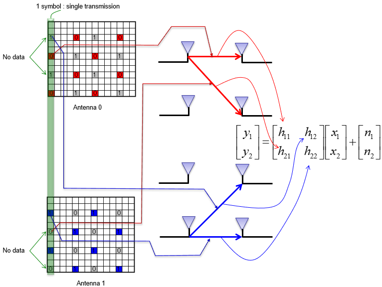
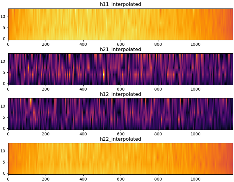
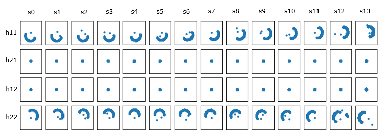
In case of SISO, the construction of channel coefficient grid is relatively simple as explained in here and here because the channel coefficient for each resource element is a scalar (a complex valued scalar). However, the channel coefficient for 2x2 MIMO is more complicated because the channel coefficient for each resource element is 2x2 matrix. How to get (construct) the 2x2 H matrix for each resource element from the two resource grid obtained in previous steps ? It is difficult to explain it verbally. The best way I can do is to express it in illustration as follows. It may not be so clear to some of you even with this illustration. Just give some time to you and think about this until it become meaningful to you. Probably thinking about the concept of channel estimation itself from the beginning may help and check out this note if you want to revisit the concept of the channel estimation.
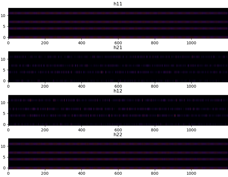
Based on the illustration shown above, I estimated channel coefficient for the resource elements of CRS (Cell specific Reference Signal) first as illustrated below. Since I have 4 elements in 2x2 Hmatrix, I got 4 resource grids showing the coefficient for the position of CRS as shown below.
|
||
