Signal Representation
As in any other field, we also use mathematical notations to represent a signal whether you like it or not -:). You should be familiar with this kind of mathematical representation since most of technical documents (especially text books) use the same expression.
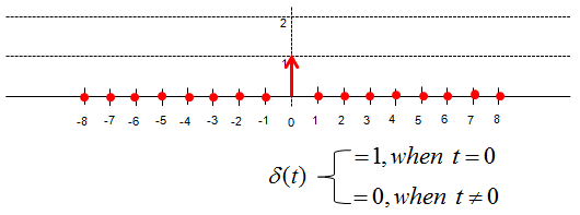
The most important component of signal representation is to understand the meaning of 'delta' fuction. Delta function in discrete signal can be illustrated as below. As you see, delta function is a special function which has '1' only at t = 0 and '0' at all other points. (In case of continuous signal, Delta function is defined as a function where the width of the function is infinitely small and the area under the function is 1).
Now let's look at a modified form of delta function. Don't worry this is the math you learned in junior high school math class.
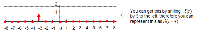
First example is as follows. I don't think you need any further explanation on this.
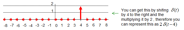
Here goes another example. I don't think you need any further explanation on this either.
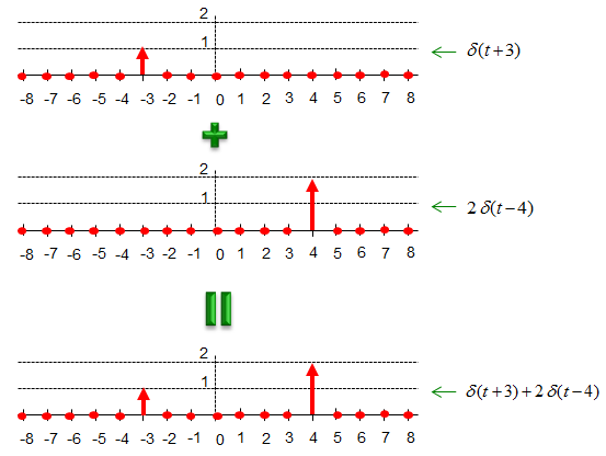
Now let's add the two modified delta function together and you would get the result as follows.
Why do we use this kind of special function and need to understand this kind of shifting/multiplication operation ?
It is because we can represent any discrete value by shift and multiplication of the function as shown below. (Note : In order for this kind of shift and multiplication to have practical meaning in real application, the system should be LTI (Linear Time Invariant). See Linearity and Time Invariance page.)
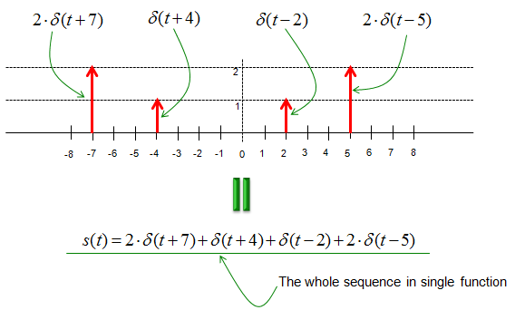
If you sum up all of these shift-multiplied versions of delta function, you can even express a sequence of signal in simple mathematical form.
If you want to express the following sequence without using the delta function, you may have to write s(t,x) = {(-8,0),(-7,2),(-6,0),(-5,0),(-4,1),(-3,0),(-2,0),(-1,0),(0,0),(1,0),(2,1),(3,0),(4,0),(5,2),(6,0),(7,0),(8,0)}. Here, t indicate time in descrete form. x indicate the amplitude (or value) of the signal at 't'. For example, s(t,x) = (-7,2) indicate the value (the amplitude of the signal) at time -7 is 2. s(t,x) = (2,1) indicate the value (the amplitude of the signal) at time 2 is 1.
Now let's think if we can s(t,x) using delta function. For example, how can we represent s(t,x) = (-7,2) using delta function ?
First, let's think of how we can represent t = -7. As described above, delta function has non-zero value only at n (time) = 0. Then how can we make the delta function has none-zero value at t = -7. With junior high school math, you can get the none zero value by shifting the delta function by 4 to the left. How can you represent this shift in math ? Again from junior high school math, you understand this can be expressed as delta(t+7).
Second, let's think of how we can represent value 2 using delta function. Again from the definition, the value of delta function at the point of none-zero value is always 1. So the value 2 can be represented as '2 x delta()'.
If you combine the result of the first and second step, you would understand s(t,x) = (-7,2) can be expressed as '2 x delta(t+7)'.
This is very important. If this is not clear to you, read this example over and over until you clearly understand this.
If you apply the same logic to each elements of s(t,x) = {(-8,0),(-7,2),(-6,0),(-5,0),(-4,1),(-3,0),(-2,0),(-1,0),(0,0),(1,0),(2,1),(3,0),(4,0),(5,2),(6,0),(7,0),(8,0)}, you can have a graph as shown below and this graph can be represented as a single mathematical expression as follows. (You would notice that I didn't indicate any points with the value 0 since it does not make any difference in final mathematical expression. But you can add the value zero part if you like. For example, you can represent (-8,0) as '0 x delta(t+8)').
Another reason why we use delta function for signal representation is the fact that the characteristics of the delta function is well investigated. Therefore, we can easily identify the characteristics of the signal based on the characteristics of the delta function. (Again, this holds true that the system is Linear Time Invarient).
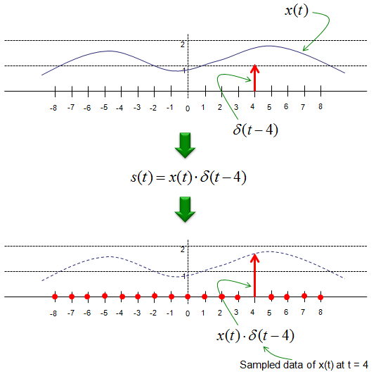
The delta function is also frequently used to represent 'sampling'. Let's say that we have a continuous signal x(t) and we want to express the value of x(t) sampled at t = 4. This can be respresented as shown below. I hope this make sense to you without any further explanation.
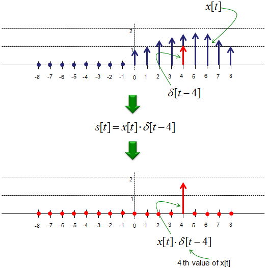
This way of representing the sampling with delta function is also applies to the discrete signal as shown below. Let's say we have a discrete signal x[t] and you want to select out the value at index 4. You can just express it as below.
This kind of mathematical expression may look unnecessarily complicated, but as I mentioned above, if you can express your signal into this kind of mathematical form you can easily characterize your signal based on a simple well known signal (delta function). One common application is to figure out the output of system when a specific input sequence is given.
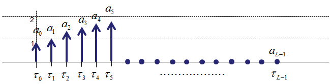
Let's go one step further. In many reading material, you would have seen a sequence of signals represented as a sequence of mathematical symbols as shown below.
![]()
This data sequence can be represented as below.
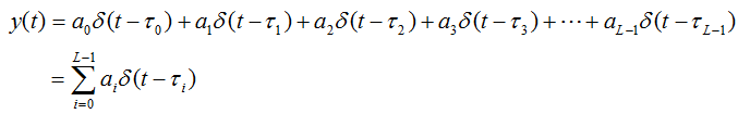
Using the delta function concept, we can represent this sequence as a single mathematical equation as below. This is the same logic as described above, but it would make it look complicated just because it is expressed in symbols rather than numbers. It is just psychological effect -:). But you have to be familiar to this kind of symbolic expression, otherwise you would have difficulties when you read papers or textbooks about communication theory.
Why we use this kind of representation ?
The main reason is that we can break down a complex system into a lot of well-known small units. Delta function is one of the well known small functions and its mathematical properties are well defined. So if we can represent a complex system into a combination of a lot of delta functions, we can characterize the mathematical properties of the complex system from the combination of the mathematical characteristics of delta function.
< Example 1 >
Here goes one example. Let's assume that you have following signal.
x[n] = [0 1 0 1 0 0 0.5 0 1 0];
and let's assume that the impulse response of the system is as follows. (By definition, impulse response is the system output for a delta input function. So this means that you already know the expected output from the system when you put a delta function as an input).
h(n) = [0 0.2 0.4 0.6 0.8 1 0.8 0.6 0.4 0.2 0];
Now, you want to predict the output from a system when you put the signal x[n] as an input. In mathematical terms, this questions is 'How to calculate the convolution of x[n] and h[n] ?'
What you can do is as follows :
i) break down the whole input sequence x[n] into each separate component using the delta function as explained above.
ii) Take the convolution of each component and the impulse response. (If you know the impulse response, you can calculate the convolution of x[t] * delta[t-n] very easily).
iii) Sum up all the results for each component you get at step ii). This sum represents the system output for your sequence as a whole.
Note : For this process to be true, the system should be LTI (Linear Time Invarient)
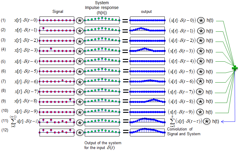
If I represent this procedure in an illustration, it would look as shown below. The original question is to find the solution shown at track (12). But it is hard to perform (and hard to understand) this at a single step. So we has broken down the problem into multiple basic forms (track (1) ~ track (10)) using the convolution of a delta function and the system and then linearly combine all of them as shown in track (11). Now you see that track (11) and track (12) shows the same result.
Many textbook would explain the meaning of system response as illustrated above, but it would not look easy and clear yet at the first look. To help you understand this concept, I put the matlab code that I used to create plots shown above. Change "x", "chan" variables as you like and see how the outcome changes. As you try this more and more, your brain would automatically draw out some general rule in your own version. (Note : You can change the value for 'x' and 'chan' anyway you like, but don't change the size of the array because I hardcoded the size of the array in for loop and number of subplots).
x = [0 1 0 1 0 0 0.5 0 1 0];
chan = [0 0.2 0.4 0.6 0.8 1 0.8 0.6 0.4 0.2 0];
chan = chan/max(chan);
y = conv(x,chan);
ysum = zeros(1,20);
for i = 1:10
tempx=zeros(1,10);
tempx(i) = x(i);
tempy = conv(tempx,chan);
ysum = ysum + tempy;
subplot(12,3,(i-1)*3+1);stem(tempx,'MarkerFaceColor',[1 0 0]);
set(gca,'xtick',[]);set(gca,'ytick',[]);axis([1 length(tempx) -1.5 1.5]);
subplot(12,3,(i-1)*3+2);stem(chan,'MarkerFaceColor',[0 1 0]);
set(gca,'xtick',[]);set(gca,'ytick',[]);axis([1 length(chan) -1.5 1.5]);
subplot(12,3,(i-1)*3+3);stem(tempy,'MarkerFaceColor',[0 0 1]);
set(gca,'xtick',[]);set(gca,'ytick',[]);axis([1 length(tempy) -1.5 1.5]);
end;
subplot(12,3,31);stem(x,'MarkerFaceColor',[1 0 0]);
set(gca,'xtick',[]);set(gca,'ytick',[]);axis([1 length(x) -1.5 1.5]);
subplot(12,3,32);stem(chan,'MarkerFaceColor',[0 1 0]);
set(gca,'xtick',[]);set(gca,'ytick',[]);axis([1 length(chan) -1.5 1.5]);
subplot(12,3,33);stem(ysum,'MarkerFaceColor',[0 0 1]);
set(gca,'xtick',[]);set(gca,'ytick',[]);axis([1 length(ysum) -max(ysum) max(ysum)]);
subplot(12,3,34);stem(x,'MarkerFaceColor',[1 0 0]);
set(gca,'xtick',[]);set(gca,'ytick',[]);axis([1 length(x) -1.5 1.5]);
subplot(12,3,35);stem(chan,'MarkerFaceColor',[0 1 0]);
set(gca,'xtick',[]);set(gca,'ytick',[]);axis([1 length(chan) -1.5 1.5]);
subplot(12,3,36);stem(y,'MarkerFaceColor',[0 0 1]);set(gca,'xtick',[]);
set(gca,'ytick',[]);axis([1 length(y) -max(y) max(y)]);
< Example 2 >
Here goes another example. Let's assume that you are asked to take the Z transform of the following signal.
x[n] = [0 1 0 1 0 0 0.5 0 1 0];
Don't worry too much about what the Z transform is. Just take the Z transform of delta and shifted delta function is defined as follows.
![]()
Now the first step is to label each of the elements and you should get very familiar with this kind of labeling.
![]()
Now let's express each elements of the sequence (signal) using delta function. It will become as follows. If this not clear to you, go back to the first part of this page and read over and over until this expression get clear to you.
![]()
And then the whole sequence can be expressed in a combination of all the delta functions as shown below. Again, if this not clear to you, go back to the first part of this page and read over and over until this expression get clear to you.
![]()
Now let's apply the Z transform rule for delta function to each elements of the sequence. It would become as follows.
![]()
Once you get the Z transform of each elements, you only have to linearly combine each elements to get the z transform of the whole sequence as shown below.
![]()
As you know, this linear combination can be expressed in simpler form as shown below.
![]()