The Laplacian matrix combines the degree matrix and the adjacency matrix into one matrix. It is the graph matrix with the most applications, from spectral clustering to consensus in sensor networks and the analysis of electrical networks. The plain form is also called the combinatorial Laplacian, to tell it apart from the normalized form. I'll give the definition, work one example, then normalize it, and finally show what its eigenvalues say about the graph.

• Definition
• Example
• Normalized Laplacian
• What the Eigenvalues Tell You

Definition

Formal definition of Laplacian is as follows.  In a Graph G, Laplacian L is defined as below, element by element. The definition assumes a simple undirected graph, so there are no loops and no edge weights.

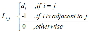
What is 'di' ? It is the diagonal elelment of 'Degree Matrix'. Actually, Laplacian can be obtained by combining the degree matrix and the adjacency matrix as follows.

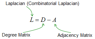
Three properties follow directly from L = D - A. First, L is symmetric, because D and A are both symmetric. Second, every row of L sums to 0. The diagonal element d_i is the number of neighbors of v_i, and the row holds exactly that many -1 values. So L1 = 0, where 1 is the vector of all ones, and 0 is always an eigenvalue of L. Third, for any vector x, x^TLx is the sum of (x_i - x_j)² over all edges. This sum can never be negative, so L is positive semidefinite and all its eigenvalues are 0 or larger.

The third property shows why L is called a Laplacian. The quantity (Lx)_i = d_ix_i - (sum of x_j over the neighbors of v_i). This is d_i times the difference between the value at v_i and the average of its neighbors. It plays the same role as the second derivative in the continuous Laplace operator, with the sign reversed. You can also build L from the signed incidence matrix B as L = B B^T.

• L = D - A : The degrees go on the diagonal, and -1 goes wherever two vertices are adjacent.
• Every row sums to 0 : So L1 = 0, and 0 is always an eigenvalue.
• x^TLx is a sum of squared differences over the edges : L is positive semidefinite, and it measures how much a signal x changes across the edges.

Example

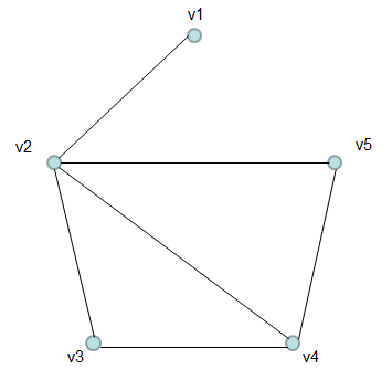
Let's assume that we have a Graph as shown below. It is the same five-vertex graph as the one on the Degree Matrix page, with the edges v1-v2, v2-v3, v2-v4, v2-v5, v3-v4 and v4-v5.

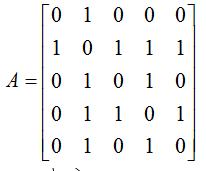
The adjacency matrix of this graph is as follows (try to build this matrix on your own as a practice).

The degree matrix of this graph is as follows (try to build this matrix on your own as a practice).

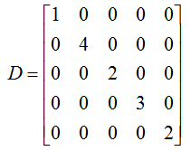
The Laplacian of this graph calculated from 'D-A' become as follows.

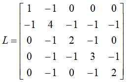
Check the row sums first. Row 2, for example, is -1 + 4 - 1 - 1 - 1 = 0, and every other row also sums to 0. The eigenvalues of this L are exactly 0, 1, 2, 4 and 5. Their sum is 12, which equals the trace of L, and the trace is the sum of the degrees. You can also check the quadratic form. With x = (1, 2, 3, 4, 5), x^TLx = 17. The same number comes from summing (x_i - x_j)² over the six edges: 1 + 1 + 4 + 9 + 1 + 1 = 17.

• Each row of the example L sums to 0 : The diagonal is the degree, and the row holds one -1 per neighbor.
• The eigenvalues are 0, 1, 2, 4 and 5 : They add up to 12, the trace of L and the sum of the degrees.
• x^TLx adds the squared differences over the edges : For x = (1, 2, 3, 4, 5) both ways give 17.

Normalized Laplacian

The combinatorial Laplacian gives more weight to vertices with many edges, because the diagonal holds the raw degree. In a graph where the degrees differ a lot, a few hub vertices can dominate the eigenvalues. The normalized Laplacian removes this effect by scaling each element with the degrees of its row and its column.

In many case, 'Normalized Laplacian' are used. The Normalized Laplacian is defined as follows. (As you see, we divide all the elements of Laplacian in such a way that the diagonal values become '1'. (di is the diagonal values on Laplacian matrix).

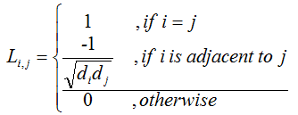
In matrix form, this is D^-1/2 L D^-1/2 = I - D^-1/2 A D^-1/2. Element (i, j) of L is divided by the square root of d_id_j. On the diagonal, that turns d_i into 1. The form needs every d_i to be positive, so an isolated vertex is treated as a special case.

Normalized Laplacian given in this example become as follows :

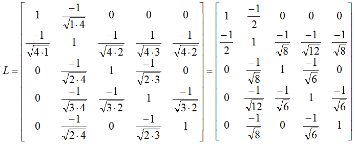
The left matrix shows each element as -1 divided by the square root of the product of the two degrees. The right matrix simplifies the roots, for example -1/√(1 x 4) = -1/2. Note that the drawing reuses the letter L for the normalized matrix. Many texts write it as L_sym or with a script L to keep the two apart. The eigenvalues of this normalized Laplacian are about 0, 0.771, 1, 1.5 and 1.729. The smallest is still 0, and none of them can be larger than 2. That fixed range is one reason the normalized form is preferred when graphs of different size are compared.

• The normalized Laplacian is D^-1/2 L D^-1/2 : Its diagonal is 1, and an edge between v_i and v_j gives -1/√(d_id_j).
• Its eigenvalues always lie between 0 and 2 : For the example they are about 0, 0.771, 1, 1.5 and 1.729.
• It needs every degree to be positive : D^-1/2 does not exist for a vertex with degree 0.

What the Eigenvalues Tell You

The main reason to build L is to read its eigenvalues. Let's sort them as λ₁ <= λ₂ <= ... <= λ_n. We already know that λ₁ = 0. The questions are how many eigenvalues are 0, how large λ₂ is, and what the eigenvectors look like.

The number of zero eigenvalues equals the number of connected components of the graph. The example has only one zero eigenvalue, so it is connected. The second smallest eigenvalue λ₂ is called the algebraic connectivity, or the Fiedler value. It is larger than 0 only when the graph is connected, and a larger value means the graph is harder to cut into two parts. For the example, λ₂ = 1.

The eigenvector of λ₂ is called the Fiedler vector, and its signs suggest where to cut the graph. For the example, the Fiedler vector is about (0.866, 0, -0.289, -0.289, -0.289). v1 has the positive sign, v2 is 0, and v3, v4 and v5 are negative. This separates v1, which hangs on a single edge, from the rest of the graph. Spectral clustering uses the same idea on large graphs.

The eigenvalues also count spanning trees. Kirchhoff's matrix tree theorem says that the number of spanning trees is the product of the nonzero eigenvalues divided by n. For the example, that is (1 x 2 x 4 x 5) / 5 = 8. The same result comes from the determinant of L with any one row and the matching column removed.

• The number of zero eigenvalues is the number of components : The example has one zero eigenvalue, so it is connected.
• λ₂ measures how well the graph is connected : For the example, the algebraic connectivity is 1.
• The signs of the Fiedler vector suggest a cut : Here they separate v1 from v3, v4 and v5.
• The nonzero eigenvalues count spanning trees : The example has (1 x 2 x 4 x 5) / 5 = 8 spanning trees.