Communication System
In this page, I will go through Matlab/Octave functions for communication system within a context of a whole process but in step-by-step manner. You would have seen many other resources elsewhere explaining on these functions, but most of the material that I have seen was purely for showing the syntax of each functions. So it was very hard for me to understand practical meaning of those functions within a whole communication process.
Following functions are the functions that is the most commonly used in Communication System.
Basic Functions
Basic Implementation of Communication Sytem.
- Creating Random BitStream
- Coverting Bit Stream into Symbol Stream
- Modulation-Mapping Symbols onto a Constellation
- Adding Noise
- Demodulation - Demapping a Constellation to a Symbol
- Converting a Symbol to Bits
- BER Calculation
- AM Modulation/Demodulation
Encoding/Decoding
- Coding(Encode/Decode)
- Galois Field
- Examples of Channel Coding
- Convolutional Code
- Examples of Representation for Convolutional Code
Channel Modeling - Matlab comm object
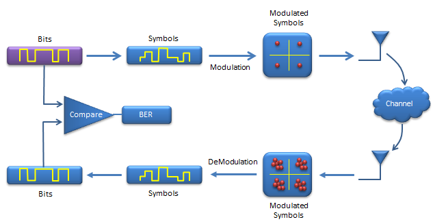
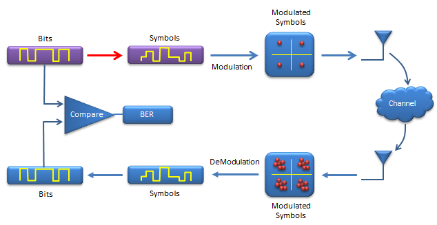
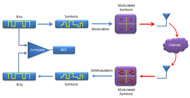
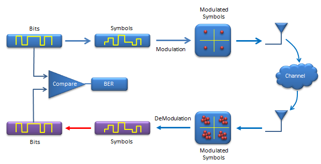
Following illustrations shows a process of a very simple (probably the simplest) communication system. Before jumping into matlab coding let's go through each steps of this process first. Before I say something, I would like each of you to step through each stage and make some story out of it.
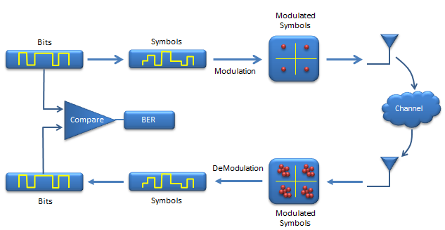
You see two tracks of the process. The upper track is 'transmission' side and lower track is 'reciever' side.
Let's look at the transmitter side first.
i) At first, you would have a digital data to transmit in the form of bits stream. (this bit stream can be one of your file, or movie or sound file or anything else).
ii) Next step is to covert this bit stream into a stream of symbols. (If you are totally new to communication system, you may not be famililar to the term called 'symbol'. Everybody would assume that you know this term, but it may not be such a simple concept. At least, it was very vague concept for me when I was first reading things about communication.. try google and understand the meaning of symbol.)
iii) Next step is to map each of those symbols on a constellation. (meaning a dot on I-Q coordinate).
iv) Next step would be to load those dots on the constellation onto a RF carrier and transmit them into the space.
v) once the signal gets into the space various kinds of noise are added to the signal and other factors distorts the signal. (The space, noise and other factors distorting the signal are called 'channel').
vi) Now the signal is received by the reciever antenna and it is down-converted and sampled. These sampled signal can be plotted onto constellation as shown above if you like.
vii) Then each of the dots on the constellation is converted to symbols.
viii) Finally each of the symbols are converted into the bit stream. (This can be a file, movie or sound that was sent by transmitter).
Following is the list of steps that I implemented with Matlab/Oactive.
- Creating Random BitStream
- Coverting Bit Stream into Symbol Stream
- Modulation-Mapping Symbols onto a Constellation
- Adding Noise
- Demodulation - Demapping a Constellation to a Symbol
- Converting a Symbol to Bits
- BER Calculation
- AM Modulation/Demodulation
Now let's look into a more complicated phase in the communication system which is about encoding/decoding for error correction. (For me, this part is the most complicated one).
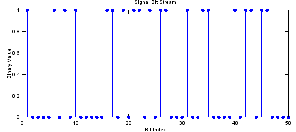
This is the first step of transmission. As I briefly described above, in real communication this can be a meaningful data like file, movie etc.. but in most of simulations or even in real life test use a sequence of random numbers (random bits) as an input data.
In Matlab/Octave, you can use any variations of rand() functions, but randint() would be the simplest one to generate the random bit stream as shown below.
Ex)
|
Input |
N = 1000; % number of data mlevel = 4; % size of signal constellation % This indicate how many constellation points you would have in I/Q plane % QAM = 4, 16 QAM = 16 etc
% signal generation in bit stream x = randint(N,1);
%plot first 50 bits stem(x(1:50),'filled'); title('Signal Bit Stream'); xlabel('Bit Index'); ylabel('Binary Value'); |
|
Output |
|
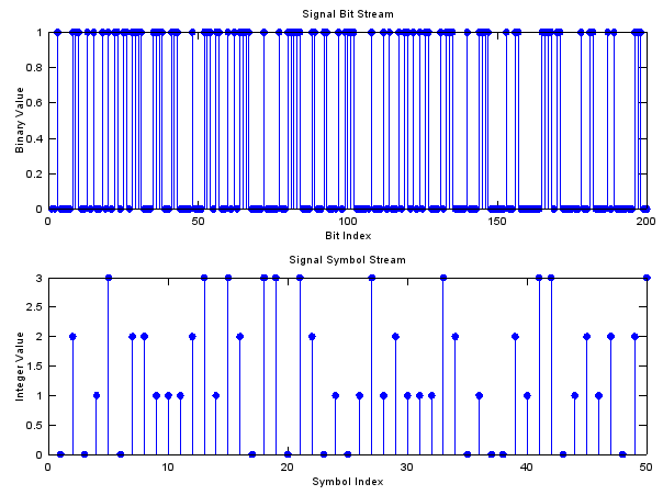
Coverting Bit Stream into Symbol Stream
Now we are converting a sequence of bits into a sequence of symbols. In this example, I will use QAM modulation, so two bits will become one symbol. ( Bit 00 -> Symbol 0, Bit 01 -> Symbol 1, Bit 10 -> Symbol 2, Bit 11 -> Symbol 3).
bi2de() function is doing this conversion. Basically it converts a sequence of bits into a corresponding decimal number. Example is shown below and compare the two plots at output.
Ex)
|
Input |
N = 1000; % number of data mlevel = 4; % size of signal constellation k = log2(mlevel); % number of bits per symbol
% signal generation in bit stream x = randint(N,1);
% convert the bit stream into symbol stream xsym = bi2de(reshape(x,k,length(x)/k).','left-msb');
%plot first 50 symbols subplot(2,1,1);stem(x(1:200),'filled'); title('Signal Bit Stream'); xlabel('Bit Index'); ylabel('Binary Value'); subplot(2,1,2);stem(xsym(1:50),'filled'); title('Signal Symbol Stream'); xlabel('Symbol Index'); ylabel('Integer Value'); |
|
Output |
|
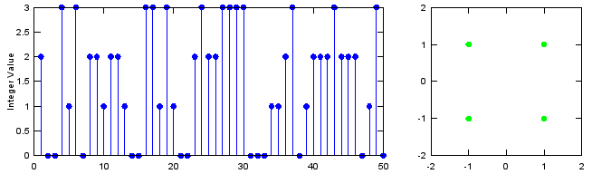
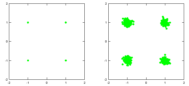
Modulation - Mapping Symbols onto a Constellation
Next step is to map each of the symbols onto constellation (dots on I/Q coordinate).
This conversion process is to create a complex number out of a symbol as shown below. It may not look intuitive with the first look. Try plugging in some numbers (e.b, -2.*mod(1,2)+2-1) and see what you get until you get clear understanding of this process.
Ex)
|
Input |
N = 1000; % number of data mlevel = 4; % size of signal constellation k = log2(mlevel); % number of bits per symbol
% signal generation in bit stream x = randint(N,1);
% convert the bit stream into symbol stream xsym = bi2de(reshape(x,k,length(x)/k).','left-msb');
% modulation b = -2.*mod(xsym,k)+k-1; a = 2.*floor(xsym./k)-k+1; xmod = a + i.*b;
%plot first 50 symbols subplot(1,3,[1 2]); stem(xsym(1:50),'filled'); title('Signal Symbol Stream'); xlabel('Symbol Index'); ylabel('Integer Value'); subplot(1,3,3); plot(real(xmod),imag(xmod),'go','MarkerFaceColor',[0,1,0]); axis([-mlevel/2 mlevel/2 -mlevel/2 mlevel/2]); |
|
Output |
|
Next step is to transmit the modulated data into the space. But there is no specific mathematical process for this transmission (even though in real system, this transmission itself also requires very complicated technology).
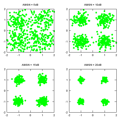
Once the signal gets into the space (channel), a variety of noise is added. For this part, you need to generate the noise part and add the noise to the signal. This two process can be done by a single function called awgn() as shown below. (You may find a lot of other sample matlab code from internet for this process in two separate steps.)
Ex)
|
Input |
N = 1000; % number of data mlevel = 4; % size of signal constellation k = log2(mlevel); % number of bits per symbol
% signal generation in bit stream x = randint(N,1);
% convert the bit stream into symbol stream xsym = bi2de(reshape(x,k,length(x)/k).','left-msb');
% modulation b = -2.*mod(xsym,k)+k-1; a = 2.*floor(xsym./k)-k+1; xmod = a + i.*b;
Tx_x = xmod;
% adding AWGN SNR = 20; Tx_awgn = awgn(Tx_x,SNR,'measured');
%plot constellation subplot(1,2,1); plot(real(Tx_x),imag(Tx_x),'go','MarkerFaceColor',[0,1,0]); axis([-mlevel/2 mlevel/2 -mlevel/2 mlevel/2]); subplot(1,2,2); plot(real(Tx_awgn),imag(Tx_awgn),'go','MarkerFaceColor',[0,1,0]); axis([-mlevel/2 mlevel/2 -mlevel/2 mlevel/2]);
SNR = 5; Tx_awgn1 = awgn(Tx_x,SNR,'measured');
SNR = 10; Tx_awgn2 = awgn(Tx_x,SNR,'measured');
SNR = 15; Tx_awgn3 = awgn(Tx_x,SNR,'measured');
SNR = 20; Tx_awgn4 = awgn(Tx_x,SNR,'measured');
%plot constellation subplot(2,2,1); plot(real(Tx_awgn1),imag(Tx_awgn1),'go','MarkerFaceColor',[0,1,0]); axis([-mlevel/2 mlevel/2 -mlevel/2 mlevel/2]);title('AWGN = 5dB'); subplot(2,2,2); plot(real(Tx_awgn2),imag(Tx_awgn2),'go','MarkerFaceColor',[0,1,0]); axis([-mlevel/2 mlevel/2 -mlevel/2 mlevel/2]);title('AWGN = 10dB'); subplot(2,2,3); plot(real(Tx_awgn3),imag(Tx_awgn3),'go','MarkerFaceColor',[0,1,0]); axis([-mlevel/2 mlevel/2 -mlevel/2 mlevel/2]);title('AWGN = 15dB'); subplot(2,2,4); plot(real(Tx_awgn4),imag(Tx_awgn4),'go','MarkerFaceColor',[0,1,0]); axis([-mlevel/2 mlevel/2 -mlevel/2 mlevel/2]);title('AWGN = 20dB'); |
|
Output |
Following is showing the signal with various strengh of noise (AWGN). Try with other values in the script until you get the practical understanding of this noise level.
|
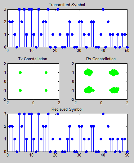
Demodulation - Demapping a Constellation to a Symbol
This step is for converting the received constellation into a symbol. Mathematically, it is to map a complex number to a corresponding symbol number. In case of QAM, qamdemod() function does this job.
Ex)
|
Input |
N = 1000; % number of data mlevel = 4; % size of signal constellation k = log2(mlevel); % number of bits per symbol
% signal generation in bit stream x = randi([0 1],N,1);
% convert the bit stream into symbol stream xsym = bi2de(reshape(x,k,length(x)/k).','left-msb');
% modulation xmod = qammod(xsym,mlevel);
Tx_x = xmod;
% adding AWGN SNR = 5; Tx_awgn = awgn(Tx_x,SNR,'measured');
% Received signal Rx_x = Tx_awgn;
%demodulation Rx_x_demod = qamdemod(Rx_x,mlevel);
%plot each steps subplot(3,2,[1 2]);stem(xsym(1:50),'filled'); title('Transmitted Symbol'); subplot(3,2,3); plot(real(Tx_x),imag(Tx_x),'go','MarkerFaceColor',[0,1,0]); axis([-mlevel/2 mlevel/2 -mlevel/2 mlevel/2]); subplot(3,2,4); plot(real(Rx_x),imag(Rx_x),'go','MarkerFaceColor',[0,1,0]); axis([-mlevel/2 mlevel/2 -mlevel/2 mlevel/2]); subplot(3,2,[5 6]);stem(Rx_x_demod(1:50),'filled'); title('Recieved Symbol'); |
|
Output |
|
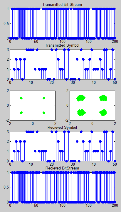
This step is for converting the symbols into Bit stream. de2bi() function do this job.
Ex)
|
Input |
N = 1000; % number of data mlevel = 4; % size of signal constellation k = log2(mlevel); % number of bits per symbol
% signal generation in bit stream x = randi([0 1],N,1);
% convert the bit stream into symbol stream xsym = bi2de(reshape(x,k,length(x)/k).','left-msb');
% modulation xmod = qammod(xsym,mlevel);
Tx_x = xmod;
% adding AWGN SNR = 5; Tx_awgn = awgn(Tx_x,SNR,'measured');
% Received signal Rx_x = Tx_awgn;
%demodulation Rx_x_demod = qamdemod(Rx_x,mlevel);
z = de2bi(Rx_x_demod,'left-msb'); % Convert integers to bits. % Convert z from a matrix to a vector. Rx_x_BitStream = reshape(z.',prod(size(z)),1);
%plot each steps subplot(5,2,[1 2]);stem(x(1:200),'filled'); title('Transmitted Bit Stream'); subplot(5,2,[3 4]);stem(xsym(1:50),'filled'); title('Transmitted Symbol'); subplot(5,2,5); plot(real(Tx_x),imag(Tx_x),'go','MarkerFaceColor',[0,1,0]); axis([-mlevel/2 mlevel/2 -mlevel/2 mlevel/2]); subplot(5,2,6); plot(real(Rx_x),imag(Rx_x),'go','MarkerFaceColor',[0,1,0]); axis([-mlevel/2 mlevel/2 -mlevel/2 mlevel/2]); subplot(5,2,[7 8]);stem(Rx_x_demod(1:50),'filled'); title('Recieved Symbol'); subplot(5,2,[9 10]);stem(Rx_x_BitStream(1:200),'filled'); title('Recieved BitStream'); |
|
Output |
|
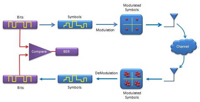
Ex)
|
Input |
N = 1000; % number of data mlevel = 4; % size of signal constellation k = log2(mlevel); % number of bits per symbol
% signal generation in bit stream x = randi([0 1],N,1);
% convert the bit stream into symbol stream xsym = bi2de(reshape(x,k,length(x)/k).','left-msb');
% modulation xmod = qammod(xsym,mlevel);
Tx_x = xmod;
% adding AWGN SNR = 5; Tx_awgn = awgn(Tx_x,SNR,'measured');
% Received signal Rx_x = Tx_awgn;
%demodulation Rx_x_demod = qamdemod(Rx_x,mlevel);
z = de2bi(Rx_x_demod,'left-msb'); % Convert integers to bits. % Convert z from a matrix to a vector. Rx_x_BitStream = reshape(z.',prod(size(z)),1);
%Calculate BER [number_of_errors,bit_error_rate] = biterr(x,Rx_x_BitStream) |
|
Output |
|
I recommend you to read Communication - Coding pages for overall concept(theoretical part) first if you are new to Coding.
gfconv(a,b,p) : a,b is a row vector representing a polynomial. p is a prime number. The result is a row vector with integer between 0 and (p-1). For example, if p is 2, the result vector is made up of binary number.
Ex) This is an example showing the code generation method explained in "Code Generation by Generator Polynomial"
|
Input |
Msg = [1 1 1 1]; GenPoly = [1 1 0 1]; codeWord = gfconv(Msg,GenPoly) |
|
Output |
codeWord = 1 0 0 1 0 1 1 |
Ex) This is an example showing the code reviewed in Overview section
|
Input |
k = 4; n = 7;
Msg = [0 0 0 0; 1 0 0 0; 0 1 0 0; 1 1 0 0; 0 0 1 0; 1 0 1 0; 0 1 1 0; 1 1 1 0; 0 0 0 1; 1 0 0 1; 0 1 0 1; 1 1 0 1; 0 0 1 1; 1 0 1 1; 0 1 1 1; 1 1 1 1] codeWord = encode(Msg,n,k,'hamming/binary') decodedMsg = decode(codeWord,n,k,'hamming/binary') |
|
Output |
Msg = 0 0 0 0 1 0 0 0 0 1 0 0 1 1 0 0 0 0 1 0 1 0 1 0 0 1 1 0 1 1 1 0 0 0 0 1 1 0 0 1 0 1 0 1 1 1 0 1 0 0 1 1 1 0 1 1 0 1 1 1 1 1 1 1
codeWord = 0 0 0 0 0 0 0 1 1 0 1 0 0 0 0 1 1 0 1 0 0 1 0 1 1 1 0 0 1 1 1 0 0 1 0 0 0 1 1 0 1 0 1 0 0 0 1 1 0 0 1 0 1 1 1 0 1 0 1 0 0 0 1 0 1 1 1 0 0 1 1 1 0 0 1 0 1 0 0 0 1 1 0 1 0 1 0 0 0 1 1 1 0 0 1 0 1 1 0 0 1 0 1 1 1 1 1 1 1 1 1 1
decodedMsg = 0 0 0 0 1 0 0 0 0 1 0 0 1 1 0 0 0 0 1 0 1 0 1 0 0 1 1 0 1 1 1 0 0 0 0 1 1 0 0 1 0 1 0 1 1 1 0 1 0 0 1 1 1 0 1 1 0 1 1 1 1 1 1 1 |
Ex)
|
Input |
m = 4; n = 2^m-1; % Codeword length = 15 k = 11; % Message length
% Create 100 messages, k bits each. Msg = randi([0,1],5,k) codeWord = encode(Msg,n,k,'hamming/binary') decodedMsg = decode(codeWord,n,k,'hamming/binary') |
|
Output |
Msg = 1 1 1 1 0 1 1 1 0 0 1 1 0 1 1 1 0 0 1 1 1 0 0 1 1 1 0 0 0 0 0 1 1 0 1 1 0 1 0 1 1 0 0 0 0 0 1 0 1 1 0 1 1 0 1
codeWord = 0 0 0 1 1 1 1 1 0 1 1 1 0 0 1 1 0 1 1 1 0 1 1 1 0 0 1 1 1 0 1 0 1 0 0 1 1 1 0 0 0 0 0 1 1 0 1 1 0 0 1 1 0 1 0 1 1 0 0 0 1 1 0 1 0 0 1 0 1 1 0 1 1 0 1
decodedMsg = 1 1 1 1 0 1 1 1 0 0 1 1 0 1 1 1 0 0 1 1 1 0 0 1 1 1 0 0 0 0 0 1 1 0 1 1 0 1 0 1 1 0 0 0 0 0 1 0 1 1 0 1 1 0 1 |
Ex) This is an example showing the code reviewed in Overview section
|
Input |
k = 4; n = 7;
Msg = [0 0 0 0; 1 0 0 0; 0 1 0 0; 1 1 0 0; 0 0 1 0; 1 0 1 0; 0 1 1 0; 1 1 1 0; 0 0 0 1; 1 0 0 1; 0 1 0 1; 1 1 0 1; 0 0 1 1; 1 0 1 1; 0 1 1 1; 1 1 1 1] codeWord = encode(Msg,n,k,'cyclic/binary') decodedMsg = decode(codeWord,n,k,'cyclic/binary') |
|
Output |
Msg = 0 0 0 0 1 0 0 0 0 1 0 0 1 1 0 0 0 0 1 0 1 0 1 0 0 1 1 0 1 1 1 0 0 0 0 1 1 0 0 1 0 1 0 1 1 1 0 1 0 0 1 1 1 0 1 1 0 1 1 1 1 1 1 1
codeWord = 0 0 0 0 0 0 0 1 1 0 1 0 0 0 0 1 1 0 1 0 0 1 0 1 1 1 0 0 1 1 1 0 0 1 0 0 0 1 1 0 1 0 1 0 0 0 1 1 0 0 1 0 1 1 1 0 1 0 1 0 0 0 1 0 1 1 1 0 0 1 1 1 0 0 1 0 1 0 0 0 1 1 0 1 0 1 0 0 0 1 1 1 0 0 1 0 1 1 0 0 1 0 1 1 1 1 1 1 1 1 1 1
decodedMsg = 0 0 0 0 1 0 0 0 0 1 0 0 1 1 0 0 0 0 1 0 1 0 1 0 0 1 1 0 1 1 1 0 0 0 0 1 1 0 0 1 0 1 0 1 1 1 0 1 0 0 1 1 1 0 1 1 0 1 1 1 1 1 1 1 |
Ex)
|
Input |
m = 4; n = 2^m-1; % Codeword length = 15 k = 11; % Message length
% Create 100 messages, k bits each. Msg = randi([0,1],5,k) codeWord = encode(Msg,n,k,'cyclic/binary') decodedMsg = decode(codeWord,n,k,'cyclic/binary') |
|
Output |
Msg = 1 0 0 1 0 0 1 0 1 0 1 0 0 1 0 1 1 1 1 0 0 0 0 0 0 0 1 0 0 0 1 0 0 0 1 1 1 0 1 0 0 1 0 1 0 1 1 1 0 0 0 1 0 1 1
codeWord = 1 0 0 1 1 0 0 1 0 0 1 0 1 0 1 0 1 0 1 0 0 1 0 1 1 1 1 0 0 0 0 1 0 1 0 0 0 0 1 0 0 0 1 0 0 1 0 1 1 0 1 1 1 0 1 0 0 1 0 1 1 1 0 1 0 1 1 1 0 0 0 1 0 1 1
decodedMsg = 1 0 0 1 0 0 1 0 1 0 1 0 0 1 0 1 1 1 1 0 0 0 0 0 0 0 1 0 0 0 1 0 0 0 1 1 1 0 1 0 0 1 0 1 0 1 1 1 0 0 0 1 0 1 1 |
Ex) This is an example of the codeword generation method explained in Generation by Generation Matrix
|
Input |
k = 4; n = 7; m = log2(n+1);
Msg = [0 0 0 0; 1 0 0 0; 0 1 0 0; 1 1 0 0; 0 0 1 0; 1 0 1 0; 0 1 1 0; 1 1 1 0; 0 0 0 1; 1 0 0 1; 0 1 0 1; 1 1 0 1; 0 0 1 1; 1 0 1 1; 0 1 1 1; 1 1 1 1]
[parmat,genmat] = hammgen(m) codeWord = encode(Msg,n,k,'linear/binary',genmat) decodedMsg = decode(codeWord,n,k,'linear/binary',genmat) |
|
Output |
Msg = 0 0 0 0 1 0 0 0 0 1 0 0 1 1 0 0 0 0 1 0 1 0 1 0 0 1 1 0 1 1 1 0 0 0 0 1 1 0 0 1 0 1 0 1 1 1 0 1 0 0 1 1 1 0 1 1 0 1 1 1 1 1 1 1
parmat = 1 0 0 1 0 1 1 0 1 0 1 1 1 0 0 0 1 0 1 1 1
genmat = 1 1 0 1 0 0 0 0 1 1 0 1 0 0 1 1 1 0 0 1 0 1 0 1 0 0 0 1
codeWord = 0 0 0 0 0 0 0 1 1 0 1 0 0 0 0 1 1 0 1 0 0 1 0 1 1 1 0 0 1 1 1 0 0 1 0 0 0 1 1 0 1 0 1 0 0 0 1 1 0 0 1 0 1 1 1 0 1 0 1 0 0 0 1 0 1 1 1 0 0 1 1 1 0 0 1 0 1 0 0 0 1 1 0 1 0 1 0 0 0 1 1 1 0 0 1 0 1 1 0 0 1 0 1 1 1 1 1 1 1 1 1 1
decodedMsg = 0 0 0 0 1 0 0 0 0 1 0 0 1 1 0 0 0 0 1 0 1 0 1 0 0 1 1 0 1 1 1 0 0 0 0 1 1 0 0 1 0 1 0 1 1 1 0 1 0 0 1 1 1 0 1 1 0 1 1 1 1 1 1 1 |
Ex) This is an example showing the way to generate arbitrary length of message and code word. This is an example of (15,11) linear block code.
|
Input |
m = 4; n = 2^m-1; % Codeword length = 15 k = 11; % Message length m = log2(n+1);
% Create 5 messages, k bits each. [parmat,genmat] = hammgen(m) Msg = randi([0,1],5,k) codeWord = encode(Msg,n,k,'linear/binary',genmat) decodedMsg = decode(codeWord,n,k,'linear/binary',genmat) |
|
Output |
parmat = 1 0 0 0 1 0 0 1 1 0 1 0 1 1 1 0 1 0 0 1 1 0 1 0 1 1 1 1 0 0 0 0 1 0 0 1 1 0 1 0 1 1 1 1 0 0 0 0 1 0 0 1 1 0 1 0 1 1 1 1
genmat = 1 1 0 0 1 0 0 0 0 0 0 0 0 0 0 0 1 1 0 0 1 0 0 0 0 0 0 0 0 0 0 0 1 1 0 0 1 0 0 0 0 0 0 0 0 1 1 0 1 0 0 0 1 0 0 0 0 0 0 0 1 0 1 0 0 0 0 0 1 0 0 0 0 0 0 0 1 0 1 0 0 0 0 0 1 0 0 0 0 0 1 1 1 0 0 0 0 0 0 0 1 0 0 0 0 0 1 1 1 0 0 0 0 0 0 0 1 0 0 0 1 1 1 1 0 0 0 0 0 0 0 0 1 0 0 1 0 1 1 0 0 0 0 0 0 0 0 0 1 0 1 0 0 1 0 0 0 0 0 0 0 0 0 0 1
Msg = 0 0 1 1 0 0 0 0 0 1 1 1 0 1 1 0 1 0 1 0 1 0 1 0 0 1 1 1 0 1 0 0 0 1 0 1 0 0 1 0 1 1 0 1 0 0 0 0 1 0 0 1 0 0 1
codeWord = 1 1 0 0 0 0 1 1 0 0 0 0 0 1 1 1 0 1 1 1 0 1 1 0 1 0 1 0 1 0 1 0 0 1 1 0 0 1 1 1 0 1 0 0 0 1 0 1 1 1 0 1 0 0 1 0 1 1 0 1 0 1 0 0 0 0 0 0 1 0 0 1 0 0 1
decodedMsg = 0 0 1 1 0 0 0 0 0 1 1 1 0 1 1 0 1 0 1 0 1 0 1 0 0 1 1 1 0 1 0 0 0 1 0 1 0 0 1 0 1 1 0 1 0 0 0 0 1 0 0 1 0 0 1
|
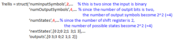
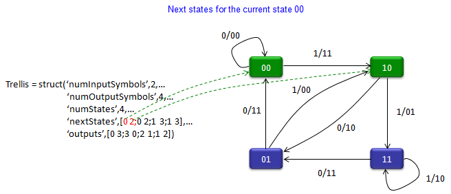
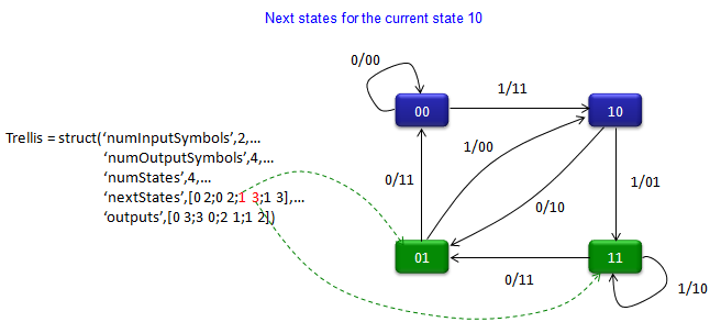
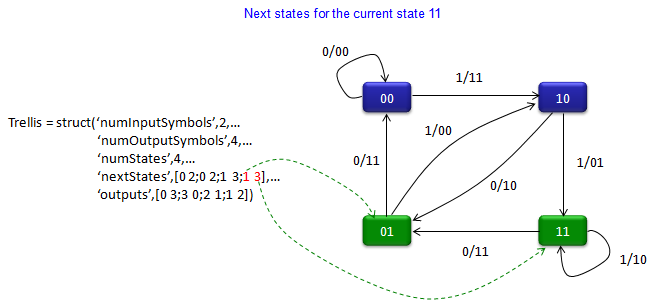
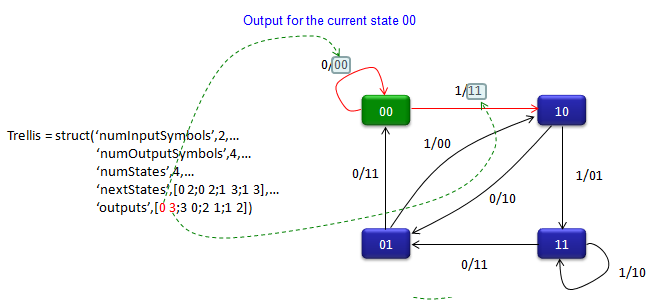
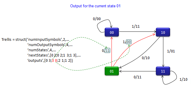
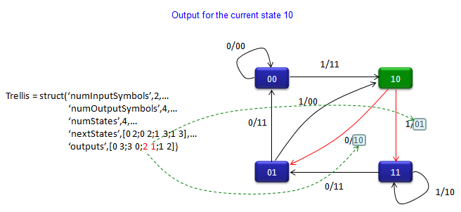
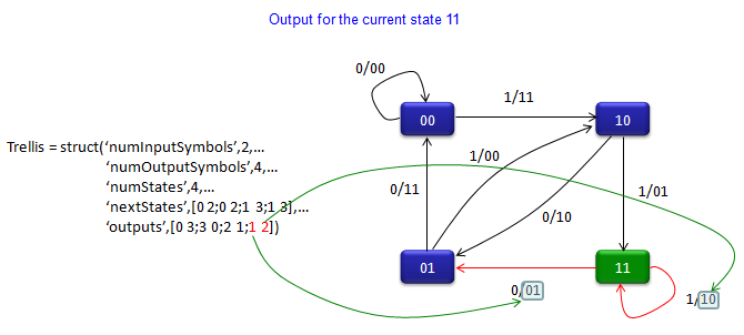
One important criteria for convolutional code would be
- Each bit on output stream is influenced not only by the current input bit but also influenced by the previous output bits.
How to represent convolutional coding process ?
Representing the convolutional coding process is not simple and clearly explained in short space. So I created a separate page for this.
Ex) You need to know how to interpret and utilize the Trellis Diagram and then get back to this example.
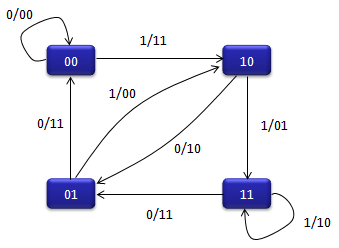
|
Input |
Trellis = struct(‘numInputSymbols’,2,… ‘numOutputSymbols’,4,… ‘numStates’,4,… ‘nextStates’,[0 2;0 2;1 3;1 3],… ‘outputs’,[0 3;3 0;2 1;1 2]) code = convenc([1 1 0 1 1],trellis) |
|
Output |
code = 1 1 0 1 0 1 0 0 0 1 |
|
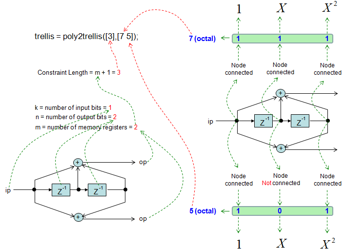
Input |
trellis = poly2trellis([3],[7 5]); code = convenc([1 1 0 1 1],trellis) |
|
Output |
code = 1 1 0 1 0 1 0 0 0 1 |
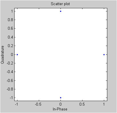
Matlab comm object has various Modulation functions and QPSKmodulator is one of them. But the QPSKModulator itself does not directly generate I/Q data. You have to use step() function to generate I/Q data. and scatterplot() to plot the IQ data
|
Input |
data = randi([0 1],100,1); hMod = comm.QPSKModulator('BitInput',true) hMod.PhaseOffset = 0; modData = step(hMod, data); scatterplot(modData) |
|
Output |
System: comm.QPSKModulator
Properties: PhaseOffset: 0.785398163397448 BitInput: true SymbolMapping: 'Gray' OutputDataType: 'double'
|
The key function in this example is 'rayleighchan()' function. This function itself does not generate IQ data for the channel. You have to use 'filter()' function and pass a input data and channel object into it to generate faded I/Q data. This examples is simple but shows almost the whole process from data generation to create faded I/Q data.
Followings are the two functions you have to know of
reyleighchan(samplingTime,
DopplerFrequencySpan,
[vector representing phase angle of each tap of the fader],
[vector representing phase gain of each tap of the fader])
filter(variable representing a channel, vector representing a list of I/Q data]
|
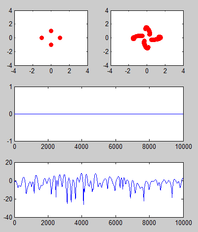
Input |
data = randi([0 1],20000,1); hMod = comm.QPSKModulator('BitInput',true) hMod.PhaseOffset = 0; modData = step(hMod, data);
channel = rayleighchan(1/1000,2,[0 2e-5 0],[0 -10 -30]) rcvData = filter(channel,modData); % Pass signal through channel
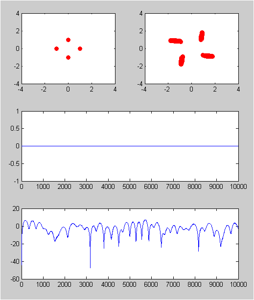
% Plot power of faded signal, versus sample number. range = 400:600; subplot(3,2,1); plot(real(modData(range)),imag(modData(range)),'ro','MarkerFaceColor',[1 0 0]); axis([-4 4 -4 4]); subplot(3,2,2); plot(real(rcvData(range)),imag(rcvData(range)),'ro','MarkerFaceColor',[1 0 0]); axis([-4 4 -4 4]); subplot(3,2,[3 4]); plot(20*log10(abs(modData))); subplot(3,2,[5 6]); plot(20*log10(abs(rcvData)));
|
|
Output |
|
The key function in this example is 'ricianchan()' function. This function itself does not generate IQ data for the channel. You have to use 'filter()' function and pass a input data and channel object into it to generate faded I/Q data. This examples is simple but shows almost the whole process from data generation to create faded I/Q data.
Followings are the two functions you have to know of
ricianchan(samplingTime,
DopplerFrequencySpan,
K)
filter(variable representing a channel, vector representing a list of I/Q data]
|
Input |
data = randi([0 1],20000,1); hMod = comm.QPSKModulator('BitInput',true) hMod.PhaseOffset = 0; modData = step(hMod, data);
channel = ricianchan(1/1000,4,1.0) rcvData = filter(channel,modData); % Pass signal through channel
% Plot power of faded signal, versus sample number. range = 400:600; subplot(3,2,1); plot(real(modData(range)),imag(modData(range)),'ro','MarkerFaceColor',[1 0 0]); axis([-4 4 -4 4]); subplot(3,2,2); plot(real(rcvData(range)),imag(rcvData(range)),'ro','MarkerFaceColor',[1 0 0]); axis([-4 4 -4 4]); subplot(3,2,[3 4]); plot(20*log10(abs(modData))); subplot(3,2,[5 6]); plot(20*log10(abs(rcvData)));
|
|
Output |
|