Signal Processing
In this page, I would post a quick reference for Matlab and Octave. (Octave is a GNU program which is designed to provide a free tool that work like Matlab. I don't think it has 100% compatability between Octave and Matlab, but I noticed that most of basic commands are compatible. I would try to list those commands that can work both with Matlab and Octave). All the sample code listed here, I tried with Octave, not with Matlab.
There are huge number of functions which has not been explained here, but I would try to list those functions which are most commonly used in most of matlab sample script you can get. My purpose is to provide you the set of basic commands with examples so that you can at least read the most of sample script you can get from here and there (e.g, internet) without overwhelming you. If you get familiar with these minimal set of functionality, you would get some 'feeling' about the tool and then you would make sense out of the official document from Mathworks or GNU Octave which explains all the functions but not so many examples.
I haven't completed 'what I think is the minimum set' yet and I hope I can complete within a couple of weeks. Stay tuned !!!
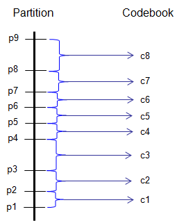
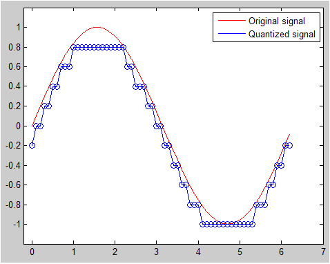
- Quantization - quantiz
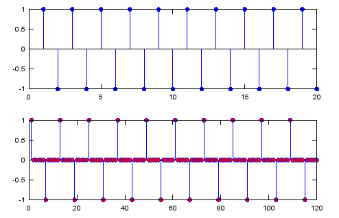
- Zero Stuffing
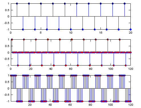
- Sample and Hold
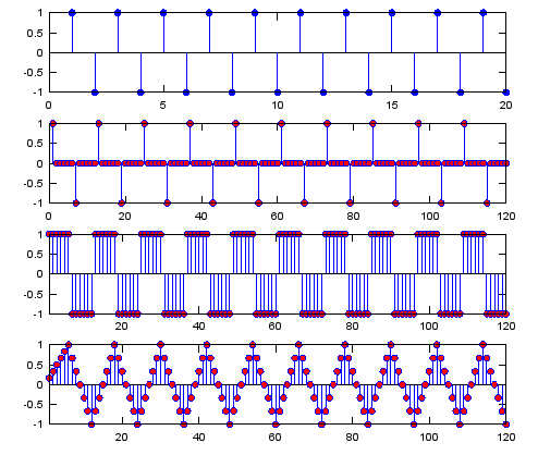
- Sample and Hold and Moving Avg
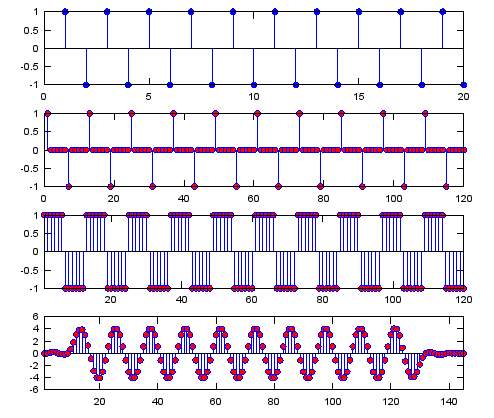
- Sample and Hold and Low Pass Filter
- interpolation - interp
- interpolation - complex number
- resample (upsample) - resample
- resample (downsample) - resample
- filter
- fir1
- fir2
- freqz
- Filter Design Tutorial
- RRC (Root Raised Cosine) Filter
Ex)
|
Input |
t = [0:.1:2*pi]; sig = sin(t); partition = [-1:.2:1]; codebook = [-1.2:.2:1]; [index,quants] = quantiz(sig,partition,codebook); plot(t,sig,'r-',t,quants,'b-',t,quants,'bo'); axis([-.2 7 -1.2 1.2]); legend('Original signal','Quantized signal'); |
|
Output |
|
Ex 1)
|
Input |
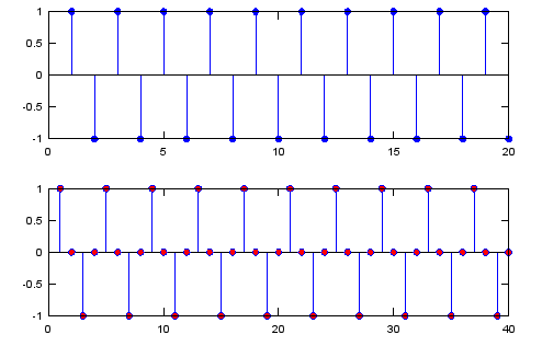
sig = [1 -1 1 -1 1 -1 1 -1 1 -1 1 -1 1 -1 1 -1 1 -1 1 -1];
sig_zerostuff = zeros(1,length(sig) * 2); sig_zerostuff(1:2:length(sig_zerostuff)) = sig;
subplot(2,1,1); stem(sig,'MarkerFaceColor',[0 0 1]); subplot(2,1,2); stem(sig_zerostuff,'MarkerFaceColor',[1 0 0]); |
|
Output |
|
Ex 2)
|
Input |
N = 6; % Upsampling Rate
sig = [1 -1 1 -1 1 -1 1 -1 1 -1 1 -1 1 -1 1 -1 1 -1 1 -1];
sig_zerostuff = zeros(1,length(sig) * N); sig_zerostuff(1:N:length(sig_zerostuff)) = sig;
subplot(2,1,1); stem(sig,'MarkerFaceColor',[0 0 1]); subplot(2,1,2); stem(sig_zerostuff,'MarkerFaceColor',[1 0 0]); |
|
Output |
|
Ex 1)
|
Input |
N = 6; % Upsampling Rate h_t = ones(1,N);
sig = [1 -1 1 -1 1 -1 1 -1 1 -1 1 -1 1 -1 1 -1 1 -1 1 -1];
sig_zerostuff = zeros(1,length(sig) * N); sig_zerostuff(1:N:length(sig_zerostuff)) = sig;
% this generate the last graph. If you are not sure how this routine can change the second graph % to the third graph, refer to 'Convolution' page first. sig_sample_hold = conv(sig_zerostuff,h_t);
subplot(3,1,1); stem(sig,'MarkerFaceColor',[0 0 1]); subplot(3,1,2); stem(sig_zerostuff,'MarkerFaceColor',[1 0 0]); subplot(3,1,3); stem(sig_sample_hold,'MarkerFaceColor',[1 0 0]);xlim([1 length(sig_zerostuff)]); |
|
Output |
|
< Sample and Hold and Moving Avg >
Ex 1)
|
Input |
N = 6; % Upsampling Rate h_t = ones(1,N); h_t_avg = (1/N) .* ones(1,N);
sig = [1 -1 1 -1 1 -1 1 -1 1 -1 1 -1 1 -1 1 -1 1 -1 1 -1];
sig_zerostuff = zeros(1,length(sig) * N); sig_zerostuff(1:N:length(sig_zerostuff)) = sig; sig_sample_hold = conv(sig_zerostuff,h_t); sig_sample_hold_avg = conv(sig_sample_hold,h_t_avg);
subplot(4,1,1); stem(sig,'MarkerFaceColor',[0 0 1]); subplot(4,1,2); stem(sig_zerostuff,'MarkerFaceColor',[1 0 0]); subplot(4,1,3); stem(sig_sample_hold,'MarkerFaceColor',[1 0 0]);xlim([1 length(sig_zerostuff)]); subplot(4,1,4); stem(sig_sample_hold_avg,'MarkerFaceColor',[1 0 0]);xlim([1 length(sig_zerostuff)]); |
|
Output |
|
< Sample and Hold and Low Pass Filter >
Ex 1)
|
Input |
N = 6; % Upsampling Rate h_t = ones(1,N); h_t_lp = sinc(-pi:2*pi/20:pi); % you can use any of low pass filter coefficient you want % I just tried to create a simple one without using signal processing % package sig = [1 -1 1 -1 1 -1 1 -1 1 -1 1 -1 1 -1 1 -1 1 -1 1 -1];
sig_zerostuff = zeros(1,length(sig) * N); sig_zerostuff(1:N:length(sig_zerostuff)) = sig; sig_sample_hold = conv(sig_zerostuff,h_t); sig_sample_hold_lp = conv(sig_sample_hold,h_t_lp);
subplot(4,1,1); stem(sig,'MarkerFaceColor',[0 0 1]); subplot(4,1,2); stem(sig_zerostuff,'MarkerFaceColor',[1 0 0]); subplot(4,1,3); stem(sig_sample_hold,'MarkerFaceColor',[1 0 0]);xlim([1 length(sig_zerostuff)]); subplot(4,1,4); stem(sig_sample_hold_lp,'MarkerFaceColor',[1 0 0]);xlim([1 length(sig_sample_hold_lp)]); |
|
Output |
|
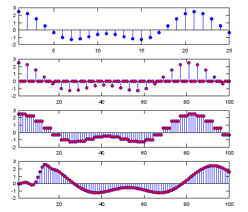
Ex 2)
: This example shows how "Interpolation" or "Upsampling" can be implemented by using 'zero stuffing' and 'low pass filter'. If you throw away the initial a couple of dozen samples of the last plot, you would see the sample plot as shown in 'interpolation' example.
|
Input |
N = 4; % Upsampling Rate h_t = ones(1,N); h_t_lp = sinc(-pi:2*pi/20:pi); h_t_lp = h_t_lp ./ sum(h_t_lp); % you can use any of low pass filter coefficient you want % I just tried to create a simple one without using signal processing % package
Fs=1000; A=1.5; B=1; f1=50; f2=100; t=0:1/Fs:1;
ti= 0:1/(Fs*N):1; sig=A*cos(2*pi*f1*t)+B*cos(2*pi*f2*t);
sig_zerostuff = zeros(1,length(sig) * N); sig_zerostuff(1:N:length(sig_zerostuff)) = sig; sig_sample_hold = conv(sig_zerostuff,h_t); sig_sample_hold_lp = conv(sig_sample_hold,h_t_lp);
subplot(4,1,1); stem(sig,'MarkerFaceColor',[0 0 1]);xlim([1 25]); subplot(4,1,2); stem(sig_zerostuff,'MarkerFaceColor',[1 0 0]);xlim([1 25*N]); subplot(4,1,3); stem(sig_sample_hold,'MarkerFaceColor',[1 0 0]);xlim([1 25*N]); subplot(4,1,4); stem(sig_sample_hold_lp,'MarkerFaceColor',[1 0 0]);xlim([1 25*N]); |
|
Output |
|
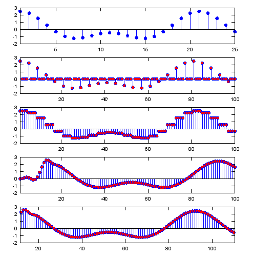
Ex 3)
: This is exactly same as Ex 2 except that it has additional graph at the last step showing some initial samples removed to show the meaningfully interpolated graph.
|
Input |
N = 4; % Upsampling Rate h_t = ones(1,N); h_t_lp = sinc(-pi:2*pi/20:pi); h_t_lp = h_t_lp ./ sum(h_t_lp); % you can use any of low pass filter coefficient you want % I just tried to create a simple one without using signal processing % package
Fs=1000; A=1.5; B=1; f1=50; f2=100; t=0:1/Fs:1;
ti= 0:1/(Fs*N):1; sig=A*cos(2*pi*f1*t)+B*cos(2*pi*f2*t);
sig_zerostuff = zeros(1,length(sig) * N); sig_zerostuff(1:N:length(sig_zerostuff)) = sig; sig_sample_hold = conv(sig_zerostuff,h_t); sig_sample_hold_lp = conv(sig_sample_hold,h_t_lp);
subplot(5,1,1); stem(sig,'MarkerFaceColor',[0 0 1]);xlim([1 25]); subplot(5,1,2); stem(sig_zerostuff,'MarkerFaceColor',[1 0 0]);xlim([1 25*N]); subplot(5,1,3); stem(sig_sample_hold,'MarkerFaceColor',[1 0 0]);xlim([1 25*N]); subplot(5,1,4); stem(sig_sample_hold_lp,'MarkerFaceColor',[1 0 0]);xlim([1 25*N]); subplot(5,1,5); stem(sig_sample_hold_lp,'MarkerFaceColor',[1 0 0]);xlim([1+length(h_t_lp)/2 25*N+length(h_t_lp)/2 |
|
Output |
|
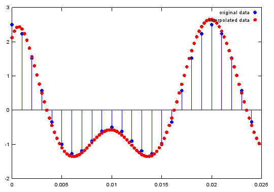
Ex)
|
Input |
Fs=1000; A=1.5; B=1; f1=50; f2=100; t=0:1/Fs:1; ifreqs=4;
ti= 0:1/(Fs*ifreqs):1; x=A*cos(2*pi*f1*t)+B*cos(2*pi*f2*t); y=interp(x,ifreqs); % interpolate signal by ifreqs
stem(t(1:25),x(1:25),'MarkerFaceColor',[0 0 1]);hold on; % plot original signal plot(ti(1:100),y(1:100),'ro','MarkerFaceColor',[1 0 0]);;hold off; legend('original data','interpolated data'); |
|
Output |
|
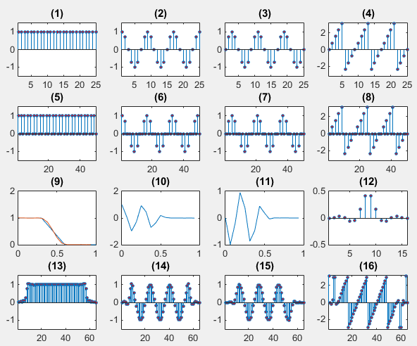
<interpolation - complex number >
Ex)
|
Input |
clear all;
t = 0:pi/4:6*pi; sig=exp(j*t);
intSig = zeros(1,2*length(sig)); intSig(1:2:end) = sig;
f = [0.0 0.3 0.6 1.0]; a = [1.0 1.0 0.0 0.0]; b = firpm(15,f,a); % this is filter design funtion with Remez Algorithm
[h,w] = freqz(b,1,16);
intFilterSig = 2 .* conv(intSig,b);
% plot original signal subplot(4,4,1); stem(abs(sig),'MarkerFaceColor',[1 0 0],'MarkerSize',3); title('(1)');xlim([1 length(sig)]);ylim([-1.5 1.5]); subplot(4,4,2); stem(real(sig),'MarkerFaceColor',[1 0 0],'MarkerSize',3); title('(2)');xlim([1 length(sig)]);ylim([-1.5 1.5]); subplot(4,4,3); stem(imag(sig),'MarkerFaceColor',[1 0 0],'MarkerSize',3); title('(3)');xlim([1 length(sig)]);ylim([-1.5 1.5]); subplot(4,4,4); stem(angle(sig),'MarkerFaceColor',[1 0 0],'MarkerSize',3); title('(4)');xlim([1 length(sig)]);ylim([-pi pi]);
% plot signal with zeros interleaved subplot(4,4,5); stem(abs(intSig),'MarkerFaceColor',[1 0 0],'MarkerSize',3); title('(5)');xlim([1 length(intSig)]); ylim([-1.5 1.5]); subplot(4,4,6); stem(real(intSig),'MarkerFaceColor',[1 0 0],'MarkerSize',3); title('(6)');xlim([1 length(intSig)]); ylim([-1.5 1.5]); subplot(4,4,7); stem(imag(intSig),'MarkerFaceColor',[1 0 0],'MarkerSize',3); title('(7)');xlim([1 length(intSig)]); ylim([-1.5 1.5]); subplot(4,4,8); stem(angle(intSig),'MarkerFaceColor',[1 0 0],'MarkerSize',3); title('(8)');xlim([1 length(intSig)]); ylim([-pi pi]);
% plot low pass filter subplot(4,4,9); plot(f,a,w/pi,abs(h));title('(9)'); subplot(4,4,10); plot(w/pi,real(h));title('(10)'); subplot(4,4,11); plot(w/pi,imag(h));title('(11)'); subplot(4,4,12); stem(b,'MarkerFaceColor',[1 0 0],'MarkerSize',3);xlim([1 length(b)]); title('(12)');
% plot signal with zeros interleaved and filtered subplot(4,4,13); stem(abs(intFilterSig),'MarkerFaceColor',[1 0 0],'MarkerSize',3); title('(13)');xlim([1 length(intFilterSig)]); ylim([-1.5 1.5]); subplot(4,4,14); stem(real(intFilterSig),'MarkerFaceColor',[1 0 0],'MarkerSize',3); title('(14)');xlim([1 length(intFilterSig)]); ylim([-1.5 1.5]); subplot(4,4,15); stem(imag(intFilterSig),'MarkerFaceColor',[1 0 0],'MarkerSize',3); title('(15)');xlim([1 length(intFilterSig)]);ylim([-1.5 1.5]); subplot(4,4,16); stem(angle(intFilterSig),'MarkerFaceColor',[1 0 0],'MarkerSize',3); title('(16)');xlim([1 length(intFilterSig)]); ylim([-pi pi]); |
|
Output |
|
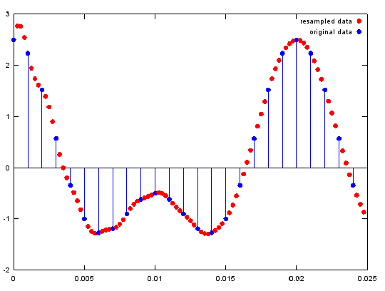
Ex)
|
Input |
Fs=1000; A=1.5; B=1; f1=50; f2=100; t=0:1/Fs:1; ifreqs=4; ti= 0:1/(Fs*ifreqs):1; x=A*cos(2*pi*f1*t)+B*cos(2*pi*f2*t); y=resample(x,ifreqs,1);
plot(ti(1:100),y(1:100),'ro','MarkerFaceColor',[1 0 0]);;hold on; stem(t(1:25),x(1:25),'MarkerFaceColor',[0 0 1]);hold off; % plot original signal legend('resampled data','original data'); |
|
Output |
|
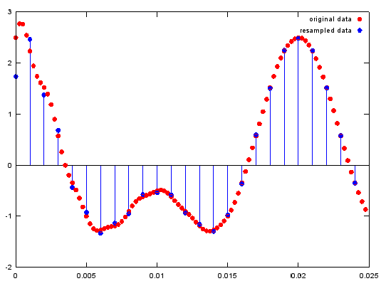
Ex)
|
Input |
Fs=1000; A=1.5; B=1; f1=50; f2=100; t=0:1/Fs:1; ifreqs=4; ti= 0:1/(Fs*ifreqs):1; x=A*cos(2*pi*f1*t)+B*cos(2*pi*f2*t);
y=resample(x,ifreqs,1);
y1=resample(y,1,ifreqs);
plot(ti(1:100),y(1:100),'ro','MarkerFaceColor',[1 0 0]);;hold on; stem(t(1:25),y1(1:25),'MarkerFaceColor',[0 0 1]);hold off; % plot original signal legend('original data','resampled data'); |
|
Output |
|
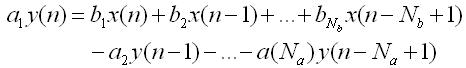
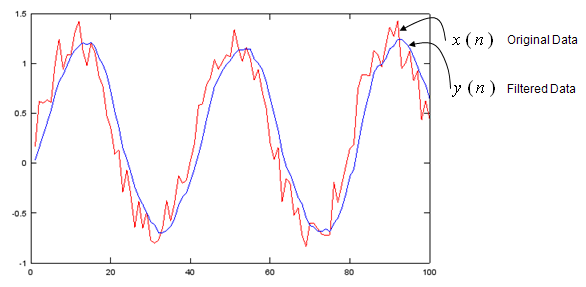
Apply the Digital Filter described as below. As you see in the mathematical description, you can apply both FIR and IIR applying the tab values.
Ex)
|
Input |
a = 1; b = [0.2 0.2 0.2 0.2 0.2]; t = linspace(0,5*pi,100); x = sin(t) .+ 0.5*rand(1,100);
y = filter(b,a,x); plot(x,'r-',y,'b-'); |
|
Output |
|
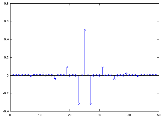
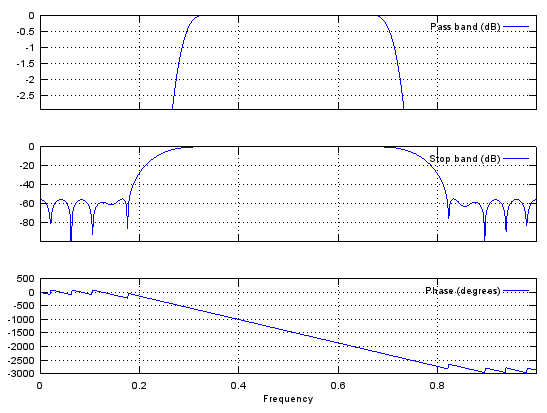
Case 1 : b = fir1(N,[pass_L,pass_R])
// Generate N tap Bandpass Filter with passband [pass_L,pass_R]. 0 < pass_L,pass_R < 1
Ex)
|
Input |
b = fir1(48,[0.25 0.75]); stem(b); figure; freqz(b,1,512); |
|
Output |
|
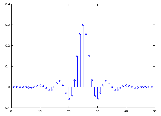
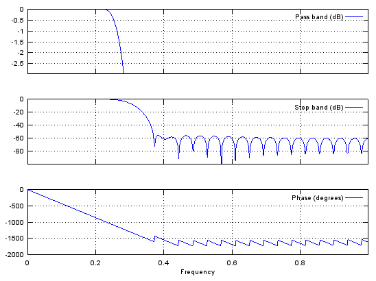
Case 2 : b = fir1(N,pass_R,'low')
// Generate N tap Lowpass Filter with passband [0,pass_R]. 0 < pass_R < 1
Ex)
|
Input |
b = fir1(48,0.3,'low'); stem(b); figure; freqz(b,1,512); |
|
Output |
|
Case 3 : b = fir1(N,pass_L,'high')
// Generate N tap Highpass Filter with passband pass_L. 0 < pass_L < 1
Ex)
|
Input |
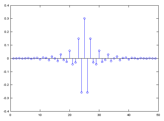
b = fir1(48,0.7,'high'); stem(b); figure; freqz(b,1,512); |
|
Output |
|
Case 4 : b = fir1(N,[stop_L stop_R],'stop')
// Generate N tap Bandstop Filter with bandstop between stop_L and stop_R. 0 < stop_L, stop_R < 1
Ex)
|
Input |
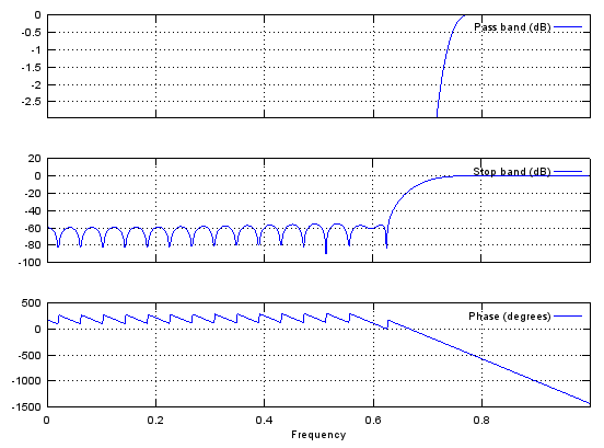
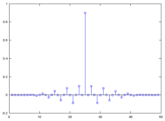
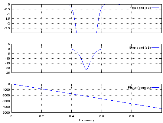
b = fir1(48,[0.45 0.55],'stop'); stem(b); figure; freqz(b,1,512); |
|
Output |
|
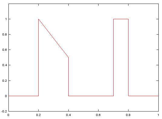
Case 1 : b = fir2(N,[f1,f2,f3,...,fm],[mag1,mag2,mag3,...,magM])
// Generate N tap Filter with aribitrary passband definition specified by [f1,f2,f3,...,fm],[mag1,mag2,mag3,...,magM]
Ex)
|
Input |
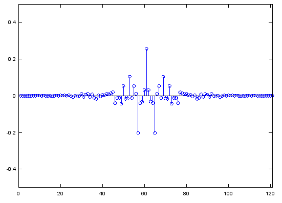
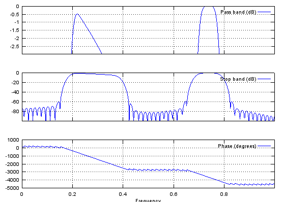
f=[0, 0.2, 0.2, 0.4, 0.4, 0.7, 0.7, 0.8, 0.8, 1]; m=[0, 0, 1, 1/2, 0, 0, 1, 1, 0, 0]; b=fir2(120,f,m);
figure; plot(f,m,'r-');axis([0 1 -0.2 1.2]); figure; stem(b);axis([0,length(b),-0.5,0.5]); figure; freqz(b,1,512); |
|
Output |
|
Case 1 : freqz(b,a,NoOfFrequencyPoints)
// Produce frequency response plot (magnitude and phase vs frequency) with IIR filter coefficient vector b and a. (In case of FIR filter, set a to be 1).
Ex)
|
Input |
b = fir1(48,[0.25 0.75]); freqz(b,1,512); |
|
Output |
|
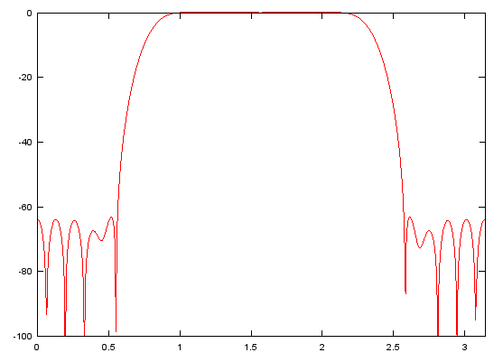
Case 2 : [h,w] = freqz(b,a,NoOfFrequencyPoints)
// return the numerical data of frequency response with IIR filter coefficient vector b and a. (In case of FIR filter, set a to be 1). h returns the magnitude values and w returns frequency point values.
Ex)
|
Input |
b = fir1(48,[0.25 0.75]); [h,w]=freqz(b,1,512); plot(w,10 .* log(abs(h)),'r-');axis([0 pi,-100,0]); |
|
Output |
|
< RRC (Root Raised Cosine) Filter >
Ex) This example may look a little complicated but the most important parts are only two lines (rcosine(), rcosflt()) as marked in blue.
|
Input |
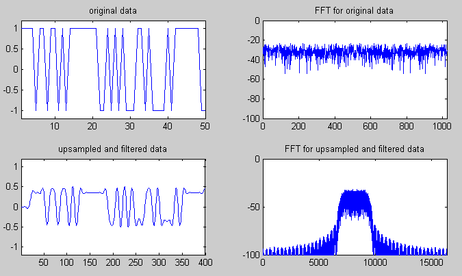
sig = randi([0 1],1024,1); % This would generate random data of {0, 1} sig = round(2*(sig - 0.5)); % This is to convert the data {0,1} into {-1,1}
upsample=8; num = rcosine(1,upsample,'sqrt'); % Transfer function of filter
% This function performs two procedures in a single step. First it upsample the input data(sig) and filter it with rrc filter (num) sig_rrc = rcosflt(sig,1,upsample,'filter',num);
% This is to perform fft. nextpow2() returns the number which is power of 2 and nearest to the number of input data. % fftshift rotate the fft data so that the peak is located at the center of the spectrum.
Lsig = length(sig); Lsig_rrc = length(sig_rrc); NFFTsig = 2^nextpow2(Lsig); NFFTsig_rrc = 2^nextpow2(Lsig_rrc); sigfft=fftshift(fft(sig,NFFTsig)/Lsig); sig_rrcfft=fftshift(fft(sig_rrc,NFFTsig_rrc)/Lsig_rrc);
% This is to convert the fft result into dB scale. sigfft_dB = 20*log10(abs(sigfft)); sig_rrcfft_dB = 20*log10(abs(sig_rrcfft));
% this is for plotting the original data and filtered data and frequency spectrum plotRange_tsig = 1:50; plotRange_tsig_rrc = 1:(50*upsample); subplot(2,2,1);plot(sig(plotRange_tsig)); axis([1 length(plotRange_tsig) -1.2 1.2]);title('original data'); subplot(2,2,2);plot(sigfft_dB); axis([0 length(sigfft_dB) -100 0]);title('FFT for original data'); subplot(2,2,3);plot(sig_rrc(plotRange_tsig_rrc)); axis([1 length(plotRange_tsig_rrc) -1.2 1.2]);title('upsampled and filtered data'); subplot(2,2,4);plot(sig_rrcfft_dB); axis([0 length(sig_rrcfft_dB) -100 0]);title('FFT for upsampled and filtered data'); |
|
Output |
|
Ex) This example may look a little complicated but the most important parts are only two lines (rcosine(), rcosflt()) as marked in blue.
|
Input |
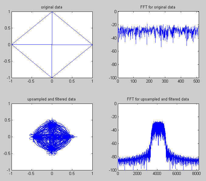
data = randi([0 1],1024,1); hMod = comm.QPSKModulator('BitInput',true) hMod.PhaseOffset = 0; sig = step(hMod, data);
upsample=8; num = rcosine(1,upsample,'sqrt'); % Transfer function of filter
% This function performs two procedures in a single step. First it upsample the input data(sig) and filter it with rrc filter (num) sig_rrc = rcosflt(sig,1,upsample,'filter',num);
% This is to perform fft. nextpow2() returns the number which is power of 2 and nearest to the number of input data. % fftshift rotate the fft data so that the peak is located at the center of the spectrum.
Lsig = length(sig); Lsig_rrc = length(sig_rrc); NFFTsig = 2^nextpow2(Lsig); NFFTsig_rrc = 2^nextpow2(Lsig_rrc); sigfft=fftshift(fft(sig,NFFTsig)/Lsig); sig_rrcfft=fftshift(fft(sig_rrc,NFFTsig_rrc)/Lsig_rrc);
% This is to convert the fft result into dB scale. sigfft_dB = 20*log10(abs(sigfft)); sig_rrcfft_dB = 20*log10(abs(sig_rrcfft));
% this is for plotting the original data and filtered data and frequency spectrum subplot(2,2,1);plot(real(sig),imag(sig)); axis([-1 1 -1 1]);title('original data'); subplot(2,2,2);plot(sigfft_dB); axis([0 length(sigfft_dB) -100 0]);title('FFT for original data'); subplot(2,2,3);plot(real(sig_rrc),imag(sig_rrc)); axis([-1 1 -1 1]);title('upsampled and filtered data'); subplot(2,2,4);plot(sig_rrcfft_dB); axis([0 length(sig_rrcfft_dB) -100 0]);title('FFT for upsampled and filtered data'); |
|
Output |
|
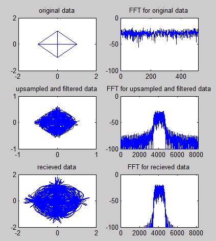
Ex) This example may look a little complicated but the most important parts are only two lines (rcosine(), rcosflt()) as marked in blue.
|
Input |
data = randi([0 1],1024,1); hMod = comm.QPSKModulator('BitInput',true) hMod.PhaseOffset = 0; sig = step(hMod, data);
upsample=8; num = rcosine(1,upsample,'sqrt'); % Transfer function of filter
% This function performs two procedures in a single step. First it upsample the input data(sig) and filter it with rrc filter (num) sig_rrc = rcosflt(sig,1,upsample,'filter',num);
sig_rcv = rcosflt(sig_rrc,1,upsample,'Fs/filter',num);
% This is to perform fft. nextpow2() returns the number which is power of 2 and nearest to the number of input data. % fftshift rotate the fft data so that the peak is located at the center of the spectrum.
Lsig = length(sig); Lsig_rrc = length(sig_rrc); Lsig_rcv = length(sig_rcv); NFFTsig = 2^nextpow2(Lsig); NFFTsig_rrc = 2^nextpow2(Lsig_rrc); NFFTsig_rcv = 2^nextpow2(Lsig_rcv); sigfft=fftshift(fft(sig,NFFTsig)/Lsig); sig_rrcfft=fftshift(fft(sig_rrc,NFFTsig_rrc)/Lsig_rrc); sig_rcvfft=fftshift(fft(sig_rcv,NFFTsig_rcv)/Lsig_rcv);
% This is to convert the fft result into dB scale. sigfft_dB = 20*log10(abs(sigfft)); sig_rrcfft_dB = 20*log10(abs(sig_rrcfft)); sig_rcvfft_dB = 20*log10(abs(sig_rcvfft));
% this is for plotting the original data and filtered data and frequency spectrum subplot(3,2,1);plot(real(sig),imag(sig)); axis([-1 1 -1 1]);title('original data'); subplot(3,2,2);plot(sigfft_dB); axis([0 length(sigfft_dB) -100 0]);title('FFT for original data'); subplot(3,2,3);plot(real(sig_rrc),imag(sig_rrc)); axis([-1 1 -1 1]);title('upsampled and filtered data'); subplot(3,2,4);plot(sig_rrcfft_dB); axis([0 length(sig_rrcfft_dB) -100 0]);title('FFT for upsampled and filtered data'); subplot(3,2,5);plot(real(sig_rcv),imag(sig_rcv)); axis([-2 2 -2 2]);title('recieved data'); subplot(3,2,6);plot(sig_rcvfft_dB); axis([0 length(sig_rcvfft_dB) -100 0]);title('FFT for recieved data'); |
|
Output |
|