Antenna is a pretty huge topic and it would be difficult to describe every aspects of Antenna in a single page, but I would try to give some big pictures of various aspects of antenna mainly for cellular application.

Let's organise the topic around three questions. What does an antenna do, how is its performance put into numbers, and how does a phone keep its antenna matched when the conditions change? The second question takes most of the page. A datasheet, a lab report and a 3GPP OTA requirement each quote a different number, so it is worth knowing exactly what each one measures.

Topics on this page are

• What is Antenna ?
• How to represent Antenna Performance ?
  • Radiation Pattern
  • Antenna Gain - G
  • Total Radiated Power - TRP
  • Total Isotropic Sensitivity - TIS
  • Effective Isotropic Radiated Power/Equivalent Isotropic Radiated Power - EIRP
  • S11
• Dynamic Antenna Matching
• References
• YouTube

What is Antenna ?

Before we measure an antenna, let's be clear about the job it does. An antenna is the place where a guided signal in a cable or a PCB trace becomes a wave in free space. A passive antenna does the same job in reverse when it receives. Every performance number later on this page describes how well one part of that conversion works.

As you know, Antenna is a device which convert Electrical Engergy (Electrical Signal) into Electromagnetic Wave which is transmitted into space.

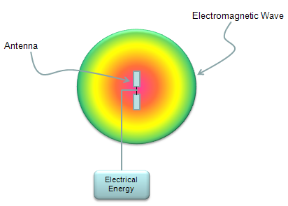
Electrical energy enters at the feed, and the antenna launches it as an electromagnetic wave into the space around it.

There are various types of antenna out there, some of the examples are shown below. These are only some examples and there are a lot of other types as well. Just check how many of these you are familiar with.

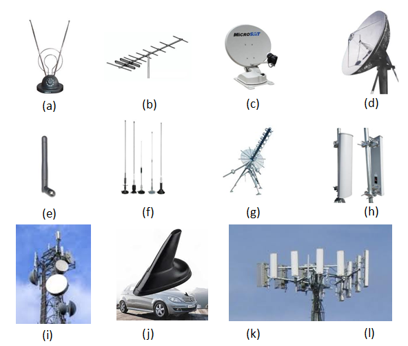
Antennas take very different shapes, because each one is built for a different band, direction and installation.

• (a) is an indoor TV antenna with two rods and a loop. (b) is a Yagi type antenna with many parallel elements on one boom.
• (c) and (d) are dish antennas. A dish concentrates the energy into one narrow direction, so it has a very high gain.
• (e) and (f) are whip antennas, the type used on routers, radios and vehicles.
• (h), (i), (k) and (l) are base station antennas: tall sector panels on masts, together with round dishes on the tower in (i).
• (j) is a shark fin antenna on the roof of a car.

Now in most of mobile communication devices, antenna are embedded in a small space. In a relatively older type of mobile phone, you might have seen the antenna shown at the left side of the picture (whip antenna). In most of the mobile devices you see these days, the antenna is embedded within the case or right on the PCB as shown below. As a mobile device (e.g, smart phone) gets more and more technologies (e.g, cellular technology with various band/radio access technology, bluetooth, WiFi etc) within a device, it is getting tougher and tougher to design multiple antenna and put them into a smal space).

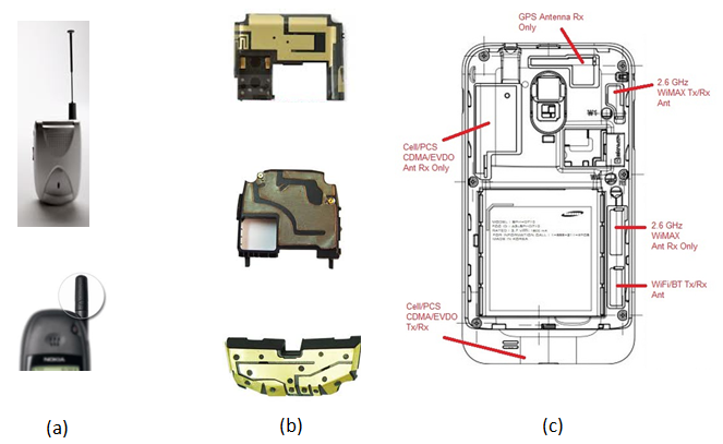
Phone antennas moved from an external whip into the housing, and one phone now carries a separate antenna for each radio.

• (a) shows older phones with an external whip or stub antenna at the top.
• (b) shows internal antenna modules. The antenna is a thin metal pattern on a small plastic carrier that sits inside the case.
• (c) shows the inside of one phone with every antenna labelled. There is a GPS Antenna Rx Only, a Cell/PCS CDMA/EVDO Tx/Rx antenna, a Cell/PCS CDMA/EVDO Ant Rx Only, a 2.6 GHz WiMAX Tx/Rx Ant, a 2.6 GHz WiMAX Ant Rx Only and a WiFi/BT Tx/Rx Ant.

Look at the labels in (c) once more. Both cellular and WiMAX have a second antenna that only receives. That second antenna is there for receive diversity, and it is the start of the multi-antenna designs used for MIMO today. So a phone has to fit several antennas, and each one has to work in its own band.

The size of the problem comes from the wavelength. The wavelength is c/f, and a simple monopole is about a quarter of a wavelength long. At 700 MHz the wavelength is about 43 cm, so a quarter wave monopole is about 10.7 cm. At 3.5 GHz the same antenna is about 2.1 cm, and at 28 GHz it is under 3 mm. This is why low bands are the hardest to fit into a phone, and why a millimeter wave phone can carry a whole array in a small module.

• An antenna converts a guided signal into a wave : a passive antenna does the same conversion in reverse when it receives.
• The antenna size follows the wavelength : a quarter wave monopole is about 10.7 cm at 700 MHz but about 2.1 cm at 3.5 GHz.
• A phone carries many antennas : separate ones for cellular, GPS, WiFi and Bluetooth, plus receive-only antennas for diversity.

How to represent Antenna Performance ?

An antenna has no single figure of merit, so the industry uses several numbers. Each number answers a different question. Comparing a gain from one datasheet with a TRP from another report is a common mistake, so let's first state the questions and then look at the numbers one by one.

There are two major criteria to evaluate Antenna Performance as follows.

i) I should convert Electrical Engergy into Electromagnetic Energy with as little loss as possible.

ii) I should be able to transmit the converted electromatic engergy as much as possible only to the direction that I want.

There are several indicators to represent the performance of an antenna as follows.

• Radiation Pattern
• Antenna Gain
• Total Radiated Power
• Total Isotropic Sensitivity

The list above names only four of them. The table below puts all six numbers of this section side by side, with the question that each one answers. Keep it in view while you read the sub-sections, because the same device can look good on one number and poor on another.

Radiation Pattern

The radiation pattern comes first, because the other numbers are either read from it or summed over it. Gain is its peak compared with an isotropic reference, and TRP is its total over the sphere.

The first step to understand/evaluate the performance of an antenna is to check the radiation pattern of the antenna. Electrical energy flows through a predefined path in most case built in a copper cable or copper trace on PCB, but once the energy is converted into electromagnetic wave, it propagate into the air almost in every direction. Depending on how we design the antenna, the direction in the air in which electromagnetic wave propagate varies. In some direction, the antenna transmit very strong energy and in some direction it transmit small amount of energy and in some direction it transmit the medium range of energy etc. This kind of engergy transmission pattern is called 'Radiation Pattern'. (For more practical example of Radiation Pattern, refer to http://rcexplorer.se/Educational/gain/gain.html )

Following is only some example of possible radiation pattern. In reality, you can think about almost infinite number of different pattern. The goal of antenna design is to make it so that it transmit the energy in the pattern that I want without any energy loss during the conversion from electrical energy to electromagnetic engergy.

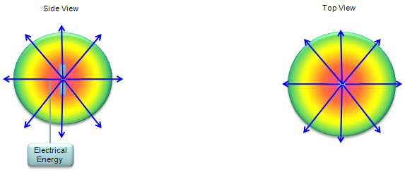
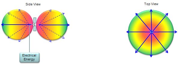
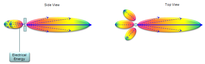
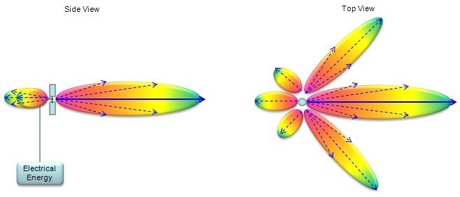
From nearly uniform to strongly directional. Each step puts more of the same energy into fewer directions.

• Each drawing has a Side View and a Top View. The arrows show the directions of radiation, and red marks the strongest part.
• Where the side view is round, the energy goes almost equally in every direction.
• Where the side view is a doughnut, there is no radiation along the axis of the antenna, and the top view is still uniform. This is the shape of a dipole. A flatter doughnut sends more energy towards the horizon.
• Where the top view shows one long main lobe with smaller side lobes and back lobes, the pattern is directional. In the pattern just above this caption, two of the other lobes are almost as long as the main lobe.

In reality, the signal radiate into 3 Dimensional Direction as illustrated (b) in the following figure. However, it is not always easy to represent the propagation patterns in 3D and sometimes it is even harder to estimate the energy propagation quantatively when it is plotted in 3D. So in many case, we cut through the 3D pattern along a specific 2D plane as shown in (c) and (d).  This plot came from Ref [7].

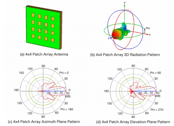
A 3D pattern is easier to read as two 2D cuts. The azimuth cut and the elevation cut together show the main beam and the side lobes.

• (a) is a 4x4 Patch Array Antenna, sixteen patches on one ground plane.
• (b) is the 3D Radiation Pattern of that array. One large main lobe points out of the front of the array, with smaller lobes around it.
• (c) is the Azimuth Plane Pattern and (d) is the Elevation Plane Pattern. Both are polar plots with a scale from -10 to 20 dB. The main lobe points to 0 deg and comes close to 20 dB, and the side lobes stay well below it.

The 20 dB peak is not a surprise. Sixteen elements that add in phase give 10log₁₀(16), about 12 dB, of array gain. Each patch has some gain of its own, and the two add in dB. The price is a narrow main beam, so the array must point that beam at the other end of the link.

• The pattern is the base of the other numbers : gain is read from its peak, and TRP is its sum over the sphere.
• A 3D pattern is usually shown as 2D cuts : the azimuth plane and the elevation plane are the two common ones.
• More elements give a narrower and stronger beam : a 4x4 array adds about 12 dB of array gain in the peak direction.

Antenna Gain - G

Gain is the number most often quoted on a datasheet, and it is also the one most often misread. The two points below explain why the word itself leads to the wrong picture.

Personally I think the 'Antenna Gain' is a misleading term because

i) When we hear the term 'Gain', we usually think 'this device would amplify a signal to make it bigger energy'. But this is not true for Antenna. Most of Antenna is 'passive device' which does not amplify anything.

ii) When we think about Gain, the higher the gain is, the higher the total amount of energy coming out of the device is. But this may not be the true in Antenna case. Higher gain in Antenna may mean "Higher engergy transmitted in a certain direction', but it may not mean 'Total amount of energy coming out of the device'.

The definition of Antenna gain is the ratio of power transmitted in a certain direction to a certain reference point. This is usually expressed in dB, dBi or dBd.  This is indicator to represent 'how well/efficiently the antenna transmit the energy in a specified direction'. Basic concept can be illustrated as follows. (For additional explanation, refer to http://rcexplorer.se/Educational/gain/gain.html )

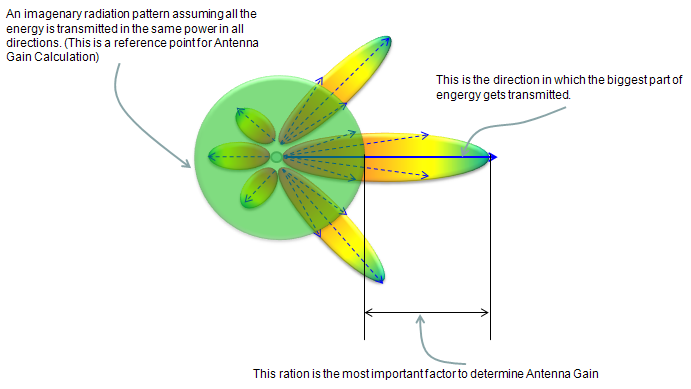
Gain compares the longest lobe with the radius of the isotropic circle that carries the same total energy.

Following is a rule of thumb propagation pattern for typical Gain values. As you see, as Antenna gain increases the direction of propagation gets more and more focused, it does not mean that the total transmission energy (the area surrounded by the ovals) gets higher.

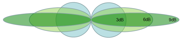
A 3 dB, a 6 dB and a 9 dB pattern. Higher gain makes the pattern longer and narrower, not larger.

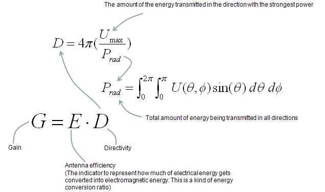
If you want to know the methmatical definition for Gain, here you go.

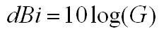
In most case, Antenna Gain is expressed in logarithmic unit as follows.

Two points in these equations are easy to miss. The first is G = E x D. Directivity D describes only the shape of the pattern. The efficiency E then removes the energy that the antenna loses as heat. So a small phone antenna can have a reasonable directivity and still a low gain, because its efficiency is low.

The second point is the reference in the unit. The unit dBi compares the antenna with an isotropic antenna. The unit dBd compares it with a half-wave dipole. A half-wave dipole has a directivity of about 1.64, which is 2.15 dBi. So a value in dBd is always 2.15 dB lower than the same value in dBi. For example, 5 dBd is 7.15 dBi. When you compare two datasheets, check this unit first.

• Gain redistributes the energy : a passive antenna cannot add power, so more energy in one direction means less in the others.
• Gain is directivity times efficiency : the shape of the pattern and the conversion loss are two separate factors.
• dBd is 2.15 dB lower than dBi : the half-wave dipole reference itself has 2.15 dBi.

Total Radiated Power - TRP

TRP answers the question that gain leaves open: how much power actually leaves the device in total. It is the number to check when a phone looks weak in every direction, not only in one. It also includes every loss between the power amplifier and free space.

It means as the term implies. It is 'sum of radiated power measured from all directions'. Simple definition of TRP can be illustrated as follows(Note : The sphere shown here is not the radiation pattern of the antenna. It is a 3 dimensional coordinate which is called 'spherical coordinate). I hope this is intuitive enough for you to get the idea without any further description.

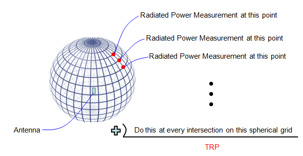
TRP is the radiated power measured at every point of a spherical grid around the antenna, and then summed.

There are two types of TRP, passive TRP and Active TRP. This classification comes from the different ways of measuring TRP. Actually it is related more to how to transmit the signal through the antenna.

In passive TRP, usually the DUT is the isolated antenna and the signal is fed directly to the antenna via the output port of a Network Analyzer (or output port of a signal generator) and measures the transmitted power through the input port of Network analyzer or input port of Spectrum Analyzer.

In active TRP, usually the DUT is the whole device including the antenna. For example, if it is for a mobile phone antenna measurement, we use the whole mobile phone as a DUT. The main purpose of Active TRP measurement is to see the performance of Antenna in real environment. In this case, you cannot use network analyzer or signal generator to transmit the signal through antenna. You have to use what most of people in this area calls a 'call box' which is basically a network simulator (e.g, eNodeB, NodeB, BTS simulator). We send the UE (e.g, mobile phone) a command 'send a signal with power XX dBm or max power' and measure the transmitted power using the 'call box' or 'spectrum analyzer'.

If you are more interested in formal expression, TRP can be represented as follows. If you are interested in how this form is derived, this page would help you.

If you like formal expression but not familiar with the meaning of this expression, following comments may help you a little bit.

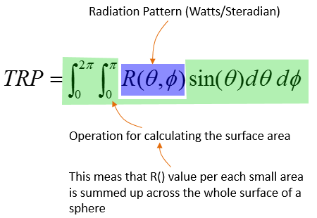
Now you might be more interested in TRP measurement as we are getting into 5G/NR. In TR 38.817-9.1.1.1, the TRP in NR is defined as follows. You see the equation is almost same as the one shown above. You see the new terminology called EIRP. In high level concept, you can take EIRP is a kind of power (not exactly same value as power, but it can directly derived from the measured power). Refer to EIRP page for further details.

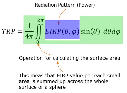
The two equations differ only in what is integrated. R(θ,φ) is power per steradian, while EIRP(θ,φ) is the power that an isotropic antenna would need to give the same signal. EIRP is therefore 4π x R, and the 1/4π in front brings the result back to the same TRP. The definition has also moved in the current specifications. In TR 38.817-02 v15.12.0, clause 9.1.1 now points to the OTA BS testing report TR 37.941, which describes the TRP measurement grids in clause 6.3.4.

In real measurement, the measurement is made at specific points across the whole surface of a spherical coordinate. So we need to convert this equation to a discrete form to get TRP from the real measurement.

If we do the measurement in a unitform grid on the coordinate, the equation can be as simple as follows :

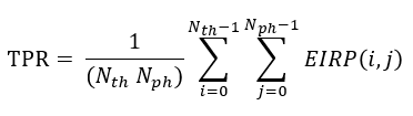
Note that the equation images on this page write TPR where they mean TRP. More importantly, this plain average is correct only when every point stands for the same area of the sphere. TR 37.941 v19.2.0 calls that a spherical equal area grid, in clause 6.3.4.3. A grid with equal steps in θ and φ is different, because its points crowd together near the poles. TR 37.941 calls that a spherical equal angle grid, in clause 6.3.4.1, and its sum is weighted by sinθ. That weighting is what the scaling factor below provides.

Let's check how large the error is. Take a dipole whose EIRP follows sin²θ, and sample it every 15 deg in θ. The true TRP is 2/3 of the peak EIRP, which is -1.76 dB. The plain average of the samples gives 0.46 of the peak, or -3.36 dB, so it is 1.6 dB too low. The weighted sum below gives 0.667, the correct value.

If the measurement is made on the non-uniform grid on the coordinate system, the equation would be as follows :

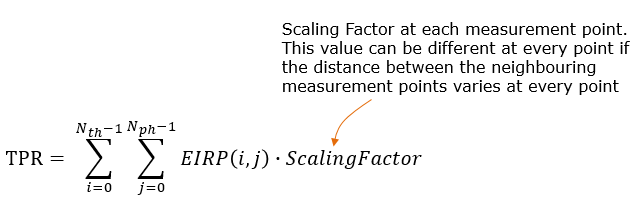
The scaling factor in this case can be derived from the area of small rectangle at the measurement point and can be expressed as shown below.

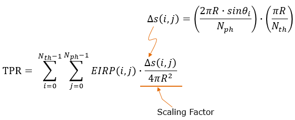
The scaling factor is the share of the sphere that one grid point covers. It contains sinθ_i, so points near the poles count less.

If you want go even deeper into the details, then you would need to refer to your Calculus textbook or refer to my note on Surface Integral example. I strongly recommend you to try to understand the details of this equation and how this is derived. It would help you a lot to understand various mathematical expressions related to antenna theory.

TRP also connects the chamber result to the conducted power. TRP in dBm is the conducted power at the antenna port plus the total efficiency of the antenna in dB, which is a negative number. For example, 23 dBm at the port and a total efficiency of -3 dB give a TRP of 20 dBm. TR 38.817-02 clause 9.2.1 writes the link to EIRP as EIRP = TRP + D in dBm, where D is the directivity in dBi.

For further reference of TRP. Refer to http://www.antenna-theory.com/definitions/trp.php

• TRP is the total radiated power : it is EIRP averaged over the whole sphere.
• Active TRP tests the whole device : the phone transmits under the control of a call box, so every loss in the phone is included.
• The grid decides the formula : an equal area grid uses a plain average, and an equal angle grid needs the sinθ weight.

Total Isotropic Sensitivity - TIS

TIS is the receive side counterpart of TRP. Instead of the power that goes out, it measures how weak a signal the device can still decode, over all directions. A lower value is better, because the device then works with a weaker signal.

First you may ask "What does 'Isotropic'mean ?"  If you look into a dictionary or google it, you would find a definition like "Identical in all direction".  TIS means "Sensitivity at every direction based on assumption that the antenna is Isotropic(radiate/receive in the same strength in all direction)".  In reality, there is no such an antenna that is purely isotropic. More practical meaning of TIS can be illustrated as below(Note : The sphere shown here is not the radiation pattern of the antenna. It is a 3 dimensional coordinate which is called 'spherical coordinate). As you see, you measure the sensitivity at every point at the intersection of a spherical grid. you wille have the different measurement result at all of those points in reality. If you take the average of those measured value, you will get a single value which indicate the TIS

TIS repeats the TRP grid on the receive side. A sensitivity search runs at every point, and the results are combined into one number.

3GPP uses the name Total Radiated Sensitivity, TRS, for the same idea. TS 37.544 v16.7.0 describes it for UTRA and E-UTRA handsets. The UE sensitivity is sampled on a sphere around it, with two orthogonal linear polarizations at each point. The step is 30 deg in both θ and φ for TRS, and 15 deg for TRP. Each sensitivity point needs a search over the downlink power, so it takes much longer than one power reading. That is a practical reason for the coarser grid.

One warning about the word average. The measured values are in dBm, but they are not averaged as dBm numbers. The spherical integration is done in linear units, like the TRP integral. So you cannot get TIS by adding the dBm values of the grid and dividing by the number of points.

For further reference of TIS. Refer to http://www.antenna-theory.com/definitions/tis.php

• TIS is sensitivity over the whole sphere : it is the receive side counterpart of TRP.
• A lower TIS is better : the device decodes a weaker signal.
• 3GPP calls it TRS : TS 37.544 samples it every 30 deg, which is coarser than the 15 deg grid for TRP.

Effective Isotropic Radiated Power/Equivalent Isotropic Radiated Power - EIRP

EIRP is the one number in this group that belongs to a single direction. It is also the number that most FR2 UE power requirements are written in, so it is worth reading carefully.

As you see the descriptions above, most of the antenna performance parameters like Gain / TRP / TIS are based on the measurement across the whole surface and some additional processing afterwards, but EIRP is a measurment showing a performance at a specific point only (i.e, the measurement at a specific angle (Phi, Theta).

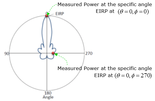
NOTE : When I say the Measured Power in above figure, it does not mean the absolute power (in dBm), it is a kind of relative power with reference to istropic power. That's why is is called Equivalent Isotropic Radiated Power. This is calculated from a couple of different parameters that can directly be measured or just given. As you see in the above figure, to accurately specify a EIRP you need to indicates the specific measurement angle. However, in many cases the term EIRP is used without specifying any specific measurement angle. In this case, it is assumed that the measurement angle is the angle where the maximum EIRP is obtained. For example, if we say EIRP of the antenna shown above without specifying any specific angle, it would me the EIRP measured at theta = 0, phy = 0.  When we assume the EIRP at the max value, it can be calculated as follows :

EIRP = Tx RF Power(dBm) + G(dB) - L(dB)

 

Tx RF Power :RF power measured at RF connector of the unit

G :Antenna gain

L : Feeder loss(cable loss or any other loss)

Let's put numbers into the formula. A base station with 46 dBm at the RF connector, a 17 dBi antenna and 3 dB of feeder loss has an EIRP of 46 + 17 - 3 = 60 dBm. Note that EIRP itself is an absolute level in dBm. It is the power that an isotropic antenna would need to produce the same signal in that direction. The relative part is the reference: the gain in dBi compares the antenna with an isotropic one.

An FR2 UE shows why one number is not enough. For power class 3 in band n257, TS 38.101-2 v20.0.0 Table 6.2.1.3-1 sets a minimum peak EIRP of 22.4 dBm. Table 6.2.1.3-2 then limits the same UE to a maximum TRP of 23 dBm and a maximum EIRP of 43 dBm. Table 6.2.1.3-3 adds spherical coverage: the EIRP at the 50th percentile of the distribution over the full sphere must be at least 11.5 dBm. So one requirement uses the peak direction, the total and the distribution over all directions.

• EIRP belongs to one direction : without a stated angle it usually means the direction of the maximum.
• EIRP is an absolute level in dBm : the isotropic reference is in the gain, not in the power.
• EIRP = TRP + D : a narrower beam raises the peak EIRP without changing the TRP.

S11

S11 is the quick check that runs before any chamber measurement. It needs only a network analyzer and a cable, so it is fast and cheap. But it answers only one of the questions in the table above.

In order to evaluate the antenna performance, we need to exactly measure the following items.

i) How much power (energy) is transmitted through the antenna without bouncing back to the input port.

ii) How much power (energy) is transmitted in the direction that I want

iii) How much weak power can be received by the antenna

Actually if you get the exact measurement for item ii) and iii), you don't need to measure item i), but to get accurate assessment for item ii) and iii), you have to perform TRP and TIS measurement as explained above. However, Measuring TRP and TIS is very expensive and time consuming. Therefore, we need some quick and simple method to evaluate the antenna performance which is to measure item i) listed above. The most common method for item i) would be to measure S11.

Since S11 shows how much energy is bounced back at the input port, the low S11 means that less energy is bounced back, implying that higher energy gets transmitted through the antenna. (Note : S11 just give you an idea of how much energy gets transmitted, but it does not give you any information on which direction the energy is transmitted. )

Let's translate S11 into lost power. S11 in dB gives the reflected share directly. At S11 = -10 dB, 10 % of the power returns to the source, and the mismatch loss is -10log₁₀(1 - 0.1) = 0.46 dB. This corresponds to a VSWR of about 1.9. At S11 = -6 dB, 25 % returns, the mismatch loss is 1.26 dB and the VSWR is about 3.0. So a poor looking S11 can cost only about 1 dB. A good S11 can still hide a large loss, because power that goes into the antenna can turn into heat instead of radiation. A 50 ohm resistor has an excellent S11 and radiates nothing.

• S11 measures only the reflection at the feed : it says nothing about direction or about loss inside the antenna.
• -10 dB S11 costs about 0.46 dB : 10 % of the power is reflected, and the VSWR is about 1.9.
• A good S11 is necessary, not sufficient : TRP and TIS in a chamber are the final check.

Dynamic Antenna Matching

A matching circuit that gave a good S11 on the bench does not stay optimal in use. A hand, a head or a table next to the phone changes the antenna impedance. A phone that covers many bands also cannot use one fixed match for all of them. This section shows how a tunable matching circuit handles both problems.

(As of Apr, 2013) I think Automatic tunning of Antenna Matching circuit is becoming a hot topic especially in mobile phone industry and think it will be a pretty common technology in near future. If you google the keywords like "Automatic Antenna Tuner","Dynamic Antenna Tuning" etc, you will find various articles, papers and patents about various tuning technology.

Basic Idea on this technology is pretty simple. (It does not tune th antennna itself, it tunes the matching circuit of the antenna).

For example, let's suppose that we have a simple Pi network type of matching circuit as shown below. (In real implementation, the matching circuit would be more complex.. but I wanted to use the simplest structure for easy understanding).

In conventional implementation, you would build as shown below. Build a circuit as follows, keep changing the values for each component until you get the best transmission of the antenna. You may find the proper values in a couple of hours if you are lucky. If you are in bad luck, you would have to spent several day-and-nights to find the proper value. If the target frequency of the antenna changes, you would have to repeat this process. and the predefined value may not always work best for all the individual antenna mass produced in the factory.

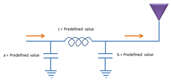
A fixed Pi network. The values a, b and c are chosen once on the bench and never change.

To solve the problems mentioned above, they came out with the concept of automatic (dynamic) tuning of the matching circuit. The baisc idea is as follows. Let's assume that we built a matching circuit with variable Inductors and variable capacitors. These variable components should not be one of those variable component you can purchase from local radio shack and set the value by rotating a knob by hand. They all should be set in electronic control to make this circuit work without human intervention. Now the tricky thing would be to find (or develope) the variable inductor and capacitors. And these variable device should operate with minimum energy (voltage, current) consumption. Currently, it would be a little bit easier to find variable capacitors than variable inductors.

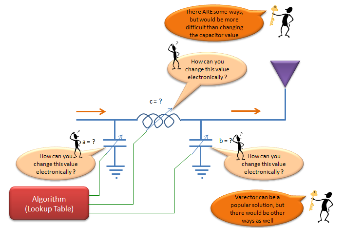
All three components become variable and are set by an algorithm. The notes point out that an inductor is more difficult to change electronically than a capacitor, and that a varactor is one option for the capacitors.

Mainly due to availability of components and some other reasons, in most auto tuning circuit we use variable capacitors as shown below. Once you build a circuit, you may have to find proper values for these components for various situations and store those values in a lookup table and the control reflash the values from the lookup table according to the situation. In this case, how to construct the proper look up table for each situation would be a critical issue.

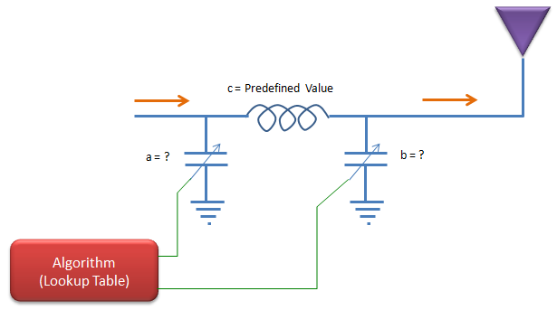
The practical open loop form. The inductor keeps a predefined value, and only the two capacitors are tuned from a lookup table.

So far so good ?

May be, or may be not.

One of the problems for the technique described above would be that you cannot guarantee the predefined look up table would work for all the possible situations. The situation may change in a little bit different way than expected and the look up table cannot do any good job. One of the common solution for this kind of situation would be to apply a value and check the result and feedback the result to the tuning algorithm so that the algorithm can do more tunings. This approach (closed loop approach) can be illustrated as shown below.

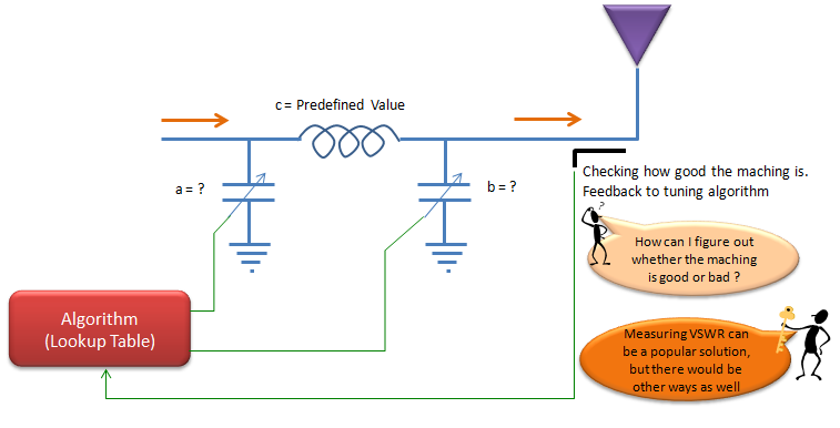
The closed loop form. A measurement at the antenna side goes back to the algorithm, so the tuner can correct a change that the lookup table did not expect.

The note in the drawing names VSWR as one way to judge the match. In practice the reflected power is sensed with a directional coupler and a power detector, and the algorithm steps the capacitor values to reduce it. Two kinds of tuning are used in phones today. Impedance tuning adjusts the matching network at the feed, as in the drawings on this page. Aperture tuning changes the antenna structure itself with a switch or a tunable capacitor, which moves its resonance to another band. The prediction in the 2013 note was correct. Tunable components are now common in smartphone antenna designs.

• A fixed match is correct only for one condition : the hand, the head and the band all change the antenna impedance.
• Open loop tuning follows a lookup table : it works for the situations that were measured in advance.
• Closed loop tuning measures the result : a reflected power reading lets the tuner correct unexpected changes.

References

[1] Wiki : Antenna

[2] AntennaTheory.com

[3] Effective Isotropic Radiated Power (EIRP)

[4] 3GPP TSG-RAN WG4 #80bis R4-167503 : BS Output power for NR

[5] EIRP Calculator

[6] Guidelines for Determining the Effective Radiated Power (ERP) and Equivalent Isotropically Radiated Power (EIRP) of a RF Transmitting System  

[7] Some Common Antenna Radiation Patterns

[8] TR 38.817-02 v15.12.0 : NR; General aspects for Base Station (BS) Radio Frequency (RF) for NR

[9] TR 37.941 v19.2.0 : Radio Frequency (RF) conformance testing background for radiated Base Station (BS) requirements

[10] TS 37.544 v16.7.0 : Universal Terrestrial Radio Access (UTRA) and Evolved Universal Terrestrial Radio Access (E-UTRA); User Equipment (UE) Over The Air (OTA) performance; Conformance testing

[11] TS 38.101-2 v20.0.0 : NR; User Equipment (UE) radio transmission and reception; Part 2: Range 2 Standalone

YouTube

• Introduction to Antennas
• Antenna Fundamentals 1 Propagation
• Antenna Fundamentals 2 Directivity
• Antenna Fundamentals 3 Bandwidth
• Antenna array part-I
• Antenna parameters
• Various forms of Antenna array
• 4.1 Antenna Basics
• 4.2 Short Dipole
• 4.3 Antenna Properties & Terminology