When I first hear of this, the first question popped in my mind was not about technical issues.. it was about english question. I thought to myself 'I think I know what 'Load' mean.. but what does it mean by 'Pull' in this case ?'.

I haven't found the exact origin of this terminology yet, it seems from googling several documents that 'pull' in this case mean 'vary (or change)'.

Therefore, 'Load Pull Test' mean 'Test something as you vary(change) the load to the DUT'.

If there is 'Load Pull', is there such a thing called 'Source Pull' ? Yes, there is and most of the test equipment for Load Pull test (Load Pull Station) can do Source Pull as well, but the term 'Source Pull' is not used frequently.

In more precise terms, the tuner sets the reflection coefficient that the DUT sees at its port. For a load impedance Z_L on a system with reference impedance Z₀, this is Γ_L = (Z_L - Z₀) / (Z_L + Z₀). For example, a 25 ohm load on a 50 ohm system gives Γ_L = -1/3, which is a VSWR of 2. Every point on the Smith Chart is one value of Γ_L. So pulling the load simply means moving the load point around the Smith Chart. This page shows the test setup first, then why the test is needed, how the results are plotted, and how a tuner creates an arbitrary impedance.

• How we test ?
• Why do this ?
• How to present the data ?
• How Load/Source Tuner works ?
• Reference

How we test ?

The detailed test setup and the required equipment would vary depending on what yo want to test (measure), but a generic test setup can be illustrated as follows.

The picture below shows the minimum bench. A network analyzer connects to a source tuner, the DUT and a load tuner in series. The source tuner sets the impedance that the DUT input sees, and the load tuner sets the impedance that the DUT output sees.

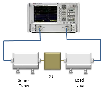
Generic load pull setup. The DUT sits between two tuners, and each tuner controls the impedance on one side of it.

As you see here, the most important thing to notice is that Tuners around the DUT. These tuners are electrical or mechanical devices that can emulate an electric circuit that can introduce any magnitude and phase. The Load for the electrical device in this setup is just a kind of electrical circuit. In terms of mathematics, the property of those electrical circuit(Load) can be expressed as single complex number with a phase component and magnitue component (In electrical terms, a Load circuit(however complicated it is) can be summarized as signle Impedance block). You can think of these  tuners as a black box that can emulate any a phase component and magnitue component.

Varying (changing) the setting in these tunner is called 'Load Pull' or 'Source Pull'.

The picture shows a network analyzer at both ends, which is the small signal view of the bench. A power load pull bench adds a signal source and a driver amplifier before the source tuner. It also adds a power meter or a spectrum analyzer after the load tuner. With these, the bench can measure output power, efficiency and ACPR at each tuner setting. The tuners themselves are characterised in advance with a network analyzer. The system stores the S-parameters of every probe position, so it knows which Γ each setting presents to the DUT.

One practical limit follows from this. Any loss between the tuner and the DUT, such as a test fixture or a cable, reduces the reflection coefficient that the DUT actually sees. The reflected wave passes through that loss twice. So a tuner that reaches |Γ| = 0.9 behind a fixture with 0.5 dB of loss presents only 0.9 x 10^-1/20 = 0.80 at the DUT. This limit matters most for power transistors, because their optimum load is often a few ohms. A 5 ohm load on a 50 ohm system needs |Γ| = 0.82, which is already beyond that 0.80.

• Each tuner setting is one reflection coefficient : the source tuner sets Γ on the input side of the DUT, and the load tuner sets Γ on the output side.
• The tuners are calibrated before the DUT is measured : the system looks up the Γ of each probe position from a stored network analyzer measurement.
• Fixture loss limits the reachable load : the loss counts twice, so 0.5 dB of loss reduces |Γ| = 0.9 at the tuner to about 0.80 at the DUT.

Why do this ?

In most of textbook situation (especially for most of passive device testing situation), what we usually do is to creating a matching circuit around the DUT that pull the load impedance to be around 50 Ohm point as in < Case A > and then measure the characteristics that you want to know at that specific point. However, for some devices (like various active devices) there are many cases where we do not use the exact 50 Ohm load for various reasons. 50 Ohm load is selected mainly because it is the best for power(energy) transfer accross the device and we need a common condition that can be agreed in the industry for easy integration of multiple discret components from various different vendors. However, this value can be good / reasonal / efficient for a certain device (e.g, passive devices) or a certain measurement parameters (e.g, S parameters), but it might not be the best condition for other types of devices(e.g, some active devices) or measurement parameters (e.g, Power efficiencies , ACPR etc).

Strictly, the 50 Ohm value itself does not give the best power transfer. Maximum power transfer happens at the conjugate match, Z_L = Z_S^*, at any impedance level. The 50 Ohm value is a compromise that comes from air-filled coaxial cable. The attenuation of such a cable is lowest at about 77 Ohm, and its power handling is highest at about 30 Ohm. 50 Ohm sits between the two, and the industry kept it as the common reference.

For a power amplifier, even the conjugate match is not the target. The conjugate match gives the highest small signal gain. At high power, the voltage swing and the maximum current of the transistor limit the output instead. The load that uses both limits fully is called the load line resistance. For an ideal device with no knee voltage, R_opt = V_DD² / (2 x P_out). A 32 V supply and 45 W of output give 32² / 90 = 11.4 ohm, and a real knee voltage makes it lower still. On a 50 ohm Smith Chart, 11.4 ohm sits at Γ = -0.63, far from the center. This is why the optimum points in the next section sit away from 50 Ohm.

Because of this kind of requirement, you need to know (measure) the characteristics of the device (DUT) at various other points at the SmithChart. Ideally at almost every points over the whole SmithChart as marked in green in < Case B >.

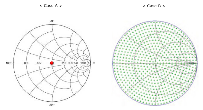
Case A measures the DUT at one load, the 50 Ohm center. Case B measures it at loads spread over the whole Smith Chart.

• In Case A, the red dot sits on the resistance axis between the labels 0.5 and 2.0, at the normalized value 1. This is the 50 Ohm point.
• In Case B, green markers cover the whole chart. Each marker is one load setting of the tuner.

• 50 Ohm is a reference, not an optimum : it is a cable compromise between low loss and high power handling, and maximum power transfer happens at the conjugate match.
• A power device wants its load line, not its conjugate match : an ideal 32 V, 45 W device needs about 11.4 ohm, far from the center of a 50 ohm chart.
• Load pull finds the optimum by measurement : the device is measured at many Γ points instead of one.

How to present the data ?

The typical way to present the load pull test data is as shown below. First, measure the test item (e.g, power, efficiency, ACPR, EVM etc) at every points (or within a certain range of the points on Smith Chart to save time) and plot it as a contour lines. Each contour line indicates that the all the load points along the contour line produces the same measurement result.

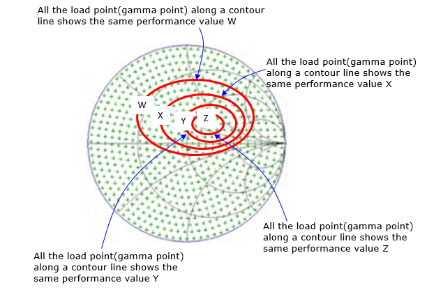
Contours of equal performance. The contours are nested, so the peak value lies inside the innermost one.

• Four red contours are labelled W, X, Y and Z from the outside in.
• Each callout reads that all the load points along one contour show the same performance value.

In many cases, you need to test the several different items (e.g, output power, efficiency, ACPR etc) for a single device. In this case, you can represent the result on multiple Smith Chart (each chart showing only one measurement item) or more commonly you can plot the multiple measurement contours on a single Smith Chart as follows. In this example, I indicated the optimal points of each of the measurement item (red, blue, black) as a smal diamond. As you see, none of them are sitting on top of exact 50 Ohm points. Also the optimal points for the items are all different. Then the question is which load condition do we need to use in the final circuit in your product to best meet the multiple characteristics ?  The answer would be 'it is up to you !'. But probably the common / most practical idia is to pick the center of the red, blue, black diamond.

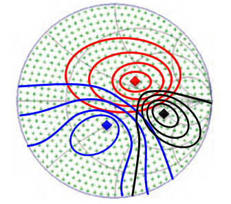
Three measurement items on one chart. Each item has its own optimum, so the final load is a compromise.

• The red diamond sits in the upper half of the chart, the blue diamond at the lower left and the black diamond to the right of the center.
• No diamond is at the center of the chart, which is the 50 Ohm point.

I would give you a more practical example of a Load pull test from a data sheet in Reference section [1]. This is just to give you an idea on some real-life example and I will leave it up to you to interpret the detailed meaning of each of the plot :)

The four charts below show one GaN transistor at 1, 2, 3 and 3.5 GHz. The red contours are P3dB, the output power at 3 dB of gain compression, in dBm. The blue contours are DrEff3dB, the drain efficiency at the same compression point, in percent. Check the scale before you read them. The resistance labels run 1, 2.5, 5, 10 and 25, and the value 5 sits at the center. So these charts are drawn around 5 ohm, not 50 ohm. This fits the load line estimate in the previous section, which put the optimum of such a device at a few ohms.

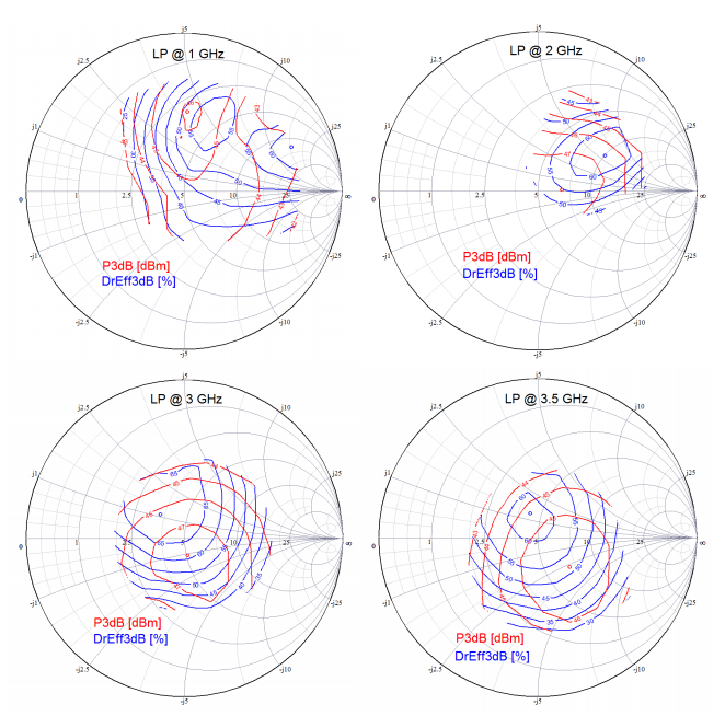
Datasheet load pull contours at four frequencies. The optimum load moves with frequency, so one matching network has to cover several optimum points.

• Each chart marks the P3dB optimum with a small red circle and the efficiency optimum with a small blue circle. The two circles never coincide.
• The red contour labels are in the low to middle 40s of dBm. The device is rated at 45 W, which is 46.5 dBm.
• At 3 GHz and 3.5 GHz, the efficiency optimum sits above the power optimum, in the inductive upper half of the chart.

I learned some tricks/tips from Taeho Kim on how to apply this Chart in every day life in Celluar RF engineering. Unfortunately I am not allowed to share the specific data for the specific application for several understandable reasons. However, the basic idea that I described in this section is based on what I learned from him.

• A contour joins loads with the same result : the peak of the measured item lies inside the innermost contour.
• Different items peak at different loads : power, efficiency and linearity each have their own optimum, so the final load is a trade-off.
• Check the chart reference impedance : power transistor datasheets often draw the chart around a few ohms, as the 5 ohm charts above do.
• The optimum moves with frequency : a wideband amplifier needs a matching network that follows the optimum across the band.

How Load/Source Tuner works ?

Many of you may not be interested in this and you don't really need to know about this.. but this was another question that came across in my mind. It was  'how can we make a general purpose circuit to create any arbitrary impedence ?' There would be several different ways to implement it, but the most typical way seems to be a kind of mechanical method as shown below. As you see, the tuner is a big box in which you can move a probe in horizontal and vertical direction. Depending on the position of the probe within the box, the total impedence of the box(tuner) varies. Now this position change can be done by Automation.

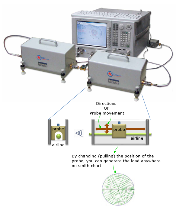
Mechanical tuner. The position of a probe over an airline sets the impedance anywhere on the Smith Chart.

• The photo shows two tuner boxes connected to a network analyzer, with the DUT between them.
• The end view shows the probe above the round center conductor of the airline.
• The side view shows the two directions of probe movement: along the airline and towards it.
• The note at the bottom says that changing (pulling) the probe position generates a load anywhere on the Smith Chart.

The two directions of the probe control the two parts of Γ. Moving the probe down towards the center conductor increases the reflection, so the vertical position mainly sets |Γ|. Moving the probe along the airline changes the line length between the DUT and the reflection point. The reflected wave travels that length twice. So a movement of d rotates the phase of Γ by 2 x β x d, where β = 2π / λ. This means a movement of half a wavelength turns Γ once around the Smith Chart. At 3.5 GHz, half a wavelength in air is 42.8 mm, and at 1 GHz it is 150 mm. So the length of the airline sets the lowest frequency at which the tuner covers the full phase range.

• The probe depth sets the magnitude : the closer the probe gets to the center conductor, the larger |Γ| becomes.
• The probe position along the airline sets the phase : a movement of half a wavelength rotates Γ by a full 360 deg.
• The airline length sets the lowest frequency : at 1 GHz the probe needs 150 mm of travel for a full turn, against 42.8 mm at 3.5 GHz.

Reference

[1] TriQuint T1G4004532-FL : 45W, 32V DC – 3.5 GHz, GaN RF Power Transistor - Datasheet  

[2] Qorvo TGF2978-SM : 20W, 32V, DC – 12 GHz, GaN RF Transistor - Datasheet