This note is based on my recent trial to decode and analyze LTE PHY signal. This is mainly to refresh my memory about the analysis process and method, but I hope it will be of help others as well.

It is not the program that process the signal real time. It was a script that I wrote in Python that process the baseband I/Q data captured from Amarisoft eNB.

NOTE : The baseband signal data (I/Q) data is captured with following condition.

• eNB and I/Q capturing device were connected with RF cable (mainly to reduce noise and get the best signal quality)
• LTE bandwidth 20 Mhz, SISO
• Sampling Rate : 30.72 MHz (Actually original capturing was done with 23.04 Mhz, but it was resampled by my script to 30.72 Mhz)

The steps below follow the order a receiver needs them. Timing comes first from the PSS, then the grid is rebuilt symbol by symbol, and only then can the CRS be used to estimate and remove the channel. The MIMO 2x2 part reuses the SISO steps and adds the channel matrix, the precoding and the large-delay CDD.

Followings are the list of procedure that I went through.

• SISO
• PSS detection
• Frequency Offset Estimation
• CP Removal - Cyclic Prefix
• Resource Grid Reconstruction
• DC Removal
• SSS Detection
• PCI Calculation
• Channel Estimation
• H grid Construction
• Equalization
• MIMO 2x2
• Resource Grid Construction - Antenna 0
• Resource Grid Construction - Antenna 1
• H Grid Construction
• Equalization
• Precoding
• Large CDD
• Reference
• Get the source code / Amarisoft TechAcademy

SISO

The SISO part takes the capture of one antenna from raw samples to a clean constellation. At 20 MHz and 30.72 MHz sampling, one 10 ms frame is 307200 samples, one OFDM symbol body is 2048 samples, and 1200 of the 2048 FFT bins carry subcarriers. Each step below uses the result of the step before it.

PSS detection

The first step to decode LTE PHY signal is to detect PSS and extract additional helper information. Personally, I think this would the most important step for LTE PHY signal processing because without this process you may not be able to decode any other signal.

This process involves multiple steps and each of those step can be a topic for separate note. For the details of nature of PSS itself and detailed algorithm to detect PSS, check out this note. In this note, I would just give you a big picture about result of PSS detection.

Following is a series of plots from my script with the detection of PSS.

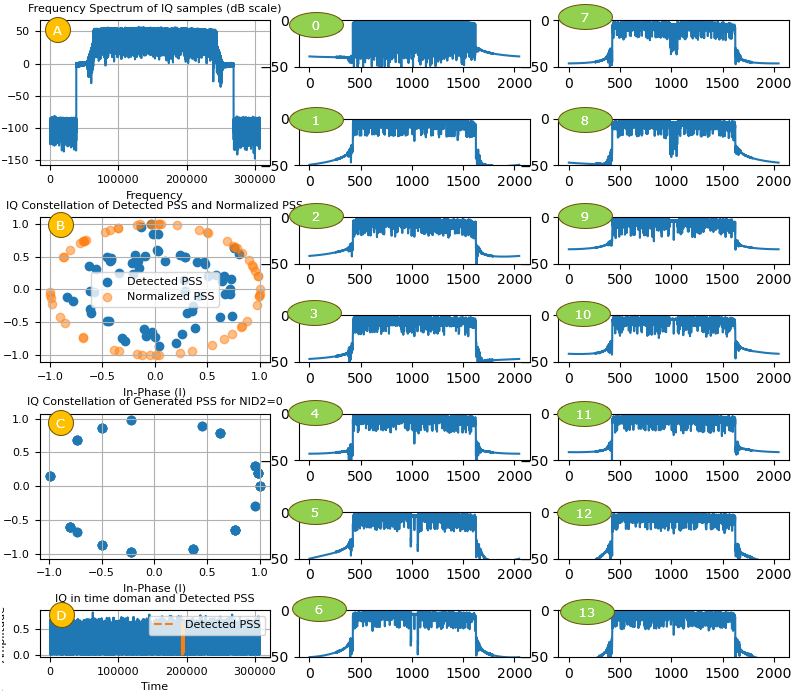
PSS detection on the 20 MHz capture. [A] is the spectrum, [B] the detected PSS as received and normalised, and [C] the PSS generated for NID2 = 0. [D] is the time-domain magnitude with the detected PSS marked, and [0] to [13] are the spectra of the 14 OFDM symbols.

[D] represents the absolute values of I/Q data. This is the plot of raw (unprocessed) data. The only process part on the plot is the part shown in orange color. It is the part on which the detected PSS is overlaid.

[A] is also a plot of non-processed data like [D]. The difference between [A] and [D] is difference between Time domain representation([D]) and Frequency Domain representation([A])

[B] is represent the detected signal (I/Q data) for PSS. The blue dots indicates the detected PSS as it is. Orange dots indicates the detected PSS projected onto the circle of radius 1. Since the blue dots does not give obvious visual correlation with the ideal PSS signal (a Zadoff sequence), I wanted to project it onto the circle like Zadoff sequence.

[C] is the ideal data that corresponds to the detected PSS data. It is the sequence generated by the script based on 3GPP spec and N_ID_2 (PSS sequence number) found during the PSS detection process.

[0]~[13] are the frequency domain plot for each OFDM symbol within the subframe where the PSS was found. Once PSS is found, we can figure out exact subframe and slot boundary of the subframe because PSS is always located in the same place (i.e, symbol 6 (7th OFDM symbol) in the subframe). With this fact, we can slice out each of OFDM data with exact start and end point. I cut out each OFDM symbols from the I/Q data and plot them in Frequency domain in dB scale.

In frame structure type 1, the PSS sits in the last OFDM symbol of slots 0 and 10. It therefore appears twice in every 10 ms frame, 5 ms apart (36.211 v19.3.0 clause 6.11.1.2). The PSS alone gives the 5 ms timing and N_ID⁽²⁾, but not which half of the frame it came from. The SSS resolves that later, because its sequence differs between subframe 0 and subframe 5. Plot [C] is titled NID2=0, so this cell uses the Zadoff-Chu root 25.

• PSS twice per frame : last symbol of slots 0 and 10.
• PSS gives N_ID⁽²⁾ : and the 5 ms timing.
• Frame timing needs the SSS : subframe 0 and 5 use different SSS sequences.

Frequency Offset Estimation

One of the important information we can get from PSS detection is frequency error (frequency offset) which can be used to adjust (correct) frequency error of other signals (e.g, correcting frequency error of SSS).

Frequency offset can be calculated / estimated as follows)

def frequency_offset_estimation(received_pss, expected_pss):

    phase_difference = np.angle(np.dot(received_pss, np.conj(expected_pss)))

    frequency_offset = phase_difference / (2 * np.pi * 62 / SampleRate)  

    return frequency_offset

The details on each line of the code is as follows :

received_pss : an array of I/Q of the detected PSS in the form of complex number

expected_pss : an array of I/Q of the PSS generated by 3GPP algorithm

def frequency_offset_estimation(received_pss, expected_pss):

    # Calculate the phase difference between the received PSS and expected PSS

    # This is achieved by first taking the dot product of the received PSS and the conjugate of the expected PSS.

    # Then, the angle (or phase) of this product is taken.

    phase_difference = np.angle(np.dot(received_pss, np.conj(expected_pss)))

    # Convert the phase difference into a frequency offset.

    # The frequency offset is calculated by dividing the phase difference by the product of:

    #   2 * pi (to convert from radians to cycles)

    #  The number of subcarriers comprising PSS  (which is 62 for LTE)

    #  dividing by the sample rate to get the offset in Hz

    frequency_offset = phase_difference / (2 * np.pi * 62 / SampleRate)

    # Return the estimated frequency offset

    return frequency_offset

NOTE :  how phase_difference / (2 * np.pi * 62 / sample_rate) can indicate the frequency offset ?

Phase and frequency are directly related: the change in phase over time is frequency. In mathematical form, it can be represented as

 dφ / dt = frequency.

In the frequency offset estimation function, the phase difference is divided by the time duration of the symbol (which is the number of subcarriers divided by the sample rate), giving us the rate of change of phase, or frequency offset.

In other words, the equation calculates the average change in phase per sample, which is then converted to Hz to represent the frequency offset. This frequency offset represents the difference in frequency between the received PSS and the expected PSS. This difference arises due to the Doppler effect or inaccuracies in the transmitter or receiver oscillators, among other reasons.

Two points about this formula are worth checking before it is reused. First, the dot product runs over the 62 PSS values of one symbol, so it measures the average phase error of that symbol, not how fast the phase changes. Second, 62 / SampleRate is the duration of 62 samples, about 2 microseconds at 30.72 MHz. One OFDM symbol body lasts 2048 samples, about 66.7 microseconds. The result is therefore a phase expressed in a frequency unit, and the scaling is a choice of this script rather than a standard estimator.

A frequency offset needs two phase measurements taken at different times. A common method uses the cyclic prefix: correlate each CP sample with the sample 2048 positions later, take the angle of the sum, and divide it by 2 x pi x 2048 / SampleRate. This estimate covers offsets from -7.5 kHz to +7.5 kHz, half the subcarrier spacing. The CP correlation page shows this correlation on real samples.

Once you get the proper frequency offset, you can compensate (correct) frequency error of other signals as follows.

signal : an array of I/Q data in the form of complex numbers.

frequency_offset : frequency offset in Hz

sample_rate : sample rate in samples / sec

def correct_frequency_offset(signal, frequency_offset, sample_rate):

    signal = np.array(signal, dtype=np.complex128)

    time = len(signal) / sample_rate

    correction = np.exp(-1j * 2 * np.pi * frequency_offset * time)

    corrected_signal = signal * correction

def correct_frequency_offset(signal, frequency_offset, sample_rate):

    # Convert the input signal into a NumPy array of complex128 data type.

    # This ensures the signal can be processed with complex arithmetic operations required for frequency correction.

    signal = np.array(signal, dtype=np.complex128)

    # Generate the time vector for the signal.

    # Instead of creating a time array that corresponds to each sample point, the code calculates the

    # total time duration of the signal by dividing its length by the sample rate.

    time = len(signal) / sample_rate

    # Calculate the complex exponential correction term.

    # This term is used to shift the signal's frequency content.

    # The negative sign in '-1j' ensures that we're shifting the frequency in the opposite direction

    # of the detected offset, thereby correcting it.

    # Multiplying by '2 * np.pi' converts the frequency offset to radians.

    correction = np.exp(-1j * 2 * np.pi * frequency_offset * time)

    # Apply the correction to the original signal by element-wise multiplication.

    # This shifts the frequency content of the signal, thereby correcting the frequency offset.

    corrected_signal = signal * correction

    return corrected_signal

The correction function has a related limit. The variable time is a single number, len(signal) / sample_rate, so correction is one complex constant and every sample is rotated by the same angle. A true frequency correction needs a phase that grows with time, which means time = np.arange(len(signal)) / sample_rate. As written, the function removes a common phase error. That is exactly what the SSS plot further down shows: the two clusters in (A) rotate onto the real axis in (B).

Any frequency error left after this step shows up again later. In the phase plot of the H grid, the line of each OFDM symbol sits a little higher than the line of the symbol before it. The channel estimation absorbs this drift, because it is measured again from the CRS in symbols 0, 4, 7 and 11.

• The dot product gives a phase : a frequency needs two measurements in time.
• CP correlation : estimates offsets from -7.5 kHz to +7.5 kHz.
• The correction is a constant rotation : time would need to be a vector of sample times.
• Residual drift : is absorbed by the CRS-based channel estimate.

CP Removal - Cyclic Prefix

Once you detected PSS and SSS, you are almost ready to reconstruct the resource grid (i.e, OFDM symbol vs Subcarrier). But before you trying to reconstruct the resource grid there is one more step to do. The time domain I/Q data carries a certain length of Cyclic Prefix (CP) data. You need to remove this part first before you reconstruct the resource grid.

The number of I/Q samples for CP varies depending on the LTE channel bandwidth as explained in this note.

36.211 v19.3.0 Table 6.12-1 gives the normal cyclic prefix as 160 T_s for the first symbol of each slot and 144 T_s for the other six, with T_s = 1/(15000 x 2048) s. At 30.72 MHz one sample lasts exactly T_s, so these lengths are 160 and 144 samples. The table below adds up one slot and one subframe.

Removing the CP means skipping 160 or 144 samples and keeping the next 2048 for the FFT. If the start is a few samples early, the window still falls inside the CP of the same symbol, and each subcarrier only picks up a phase ramp. If the start is late, the window takes samples from the next symbol, and inter-symbol interference appears.

• CP of 160 and 144 samples : at 30.72 MHz, from Table 6.12-1.
• 2048 samples per symbol body : 15360 samples per slot.
• An early window is harmless : a late one causes inter-symbol interference.

Resource Grid Reconstruction

Once you have accuarate detection of timing and frequency boundary and removed CP properly, you can construct a LTE resource grid as follows. Once you have this kind of accurate resource grid, the retrieving and generating Physical layer data is something like reading and writing numbers in an Excel spreadsheet.

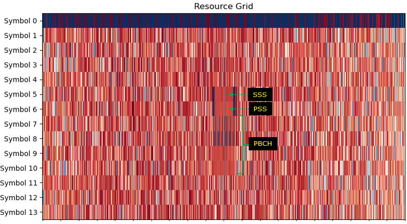
Resource grid of one subframe, 14 OFDM symbols by 1200 subcarriers. The SSS in symbol 5, the PSS in symbol 6 and the PBCH in symbols 7 to 10 occupy the central 72 subcarriers.

Each row of the grid is the FFT of one 2048-sample symbol body, reduced to the 1200 bins that carry the 100 RB. The labels match 36.211: the PBCH takes the first four symbols of slot 1 on the central 6 RB (clause 6.6.4), and the PBCH is sent only in subframe 0. This grid is therefore subframe 0. Symbol 0 holds the control region, and its colour differs from the data symbols below it.

DC Removal

There is still one more step to do after you reconstructed the ResourceGrid after CP removal. It is the process of an subcarrier at the center of the resource grid.

In the LTE downlink, the subcarrier at the carrier frequency is not used. The baseband formula in 36.211 v19.3.0 clause 6.12 sums over subcarrier indices from -600 to -1 and from 1 to 600 at 20 MHz, and skips index 0. After the 2048-point FFT, the receiver keeps 600 bins below DC and 600 bins above it, and drops the DC bin itself. If the DC bin were kept, every subcarrier on the upper side would move by one position, and the CRS positions would no longer match.

Dropping the DC bin also removes the local oscillator leakage that a direct-conversion receiver can leave at that frequency. The resource grid then holds exactly 1200 subcarriers, numbered from 0 at the lowest frequency.

• The DC subcarrier carries nothing : 36.211 clause 6.12 skips index 0.
• Keep 600 bins on each side : 1200 subcarriers at 20 MHz.
• Keeping the DC bin : shifts the upper half by one subcarrier.

SSS Detection

Once you able to construct an accurate resource grid as shown above, the first thing you need to do is to detect SSS(Secondary Synchronized Signal). This process is done as in the following step :

i) Retrieve I/Q data from the resource elements for SSS from the Resource Grid

ii) Compensate the retrieved SSS I/Q with frequency offset obtained by PSS detection procedure.

iii) Generate all the possible SSS sequence that belong to the category for N_ID_2 (PSS sequence number)

iv) Compare (correlate) each and every SSS sequence from step iii) with the SSS IQ data from step ii) and find the best pair. The SSS sequence index (N_ID_1) that gives the best correlation is the detected SSS.

NOTE : The procedure for step iii) and iv) is explained in detail in this note.

Some highlights of SSS detection procedure are plotted below. (A) is the original IQ data retrieved from the resource grid(this corresponds to step i) mentioned above). (B) is the SSS data compensated by frequency offset (this corresponds to step ii) mentioned above). (C) is just one example of the generated SSS (this corresponds to step iii) mentioned above)

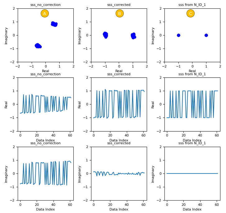
SSS detection. (A) the SSS as read from the grid, (B) after the phase correction, (C) the SSS generated for the detected N_ID_1. Each column shows the constellation, the real part and the imaginary part.

The SSS is a real sequence of +1 and -1 values on 62 subcarriers (36.211 v19.3.0 clause 6.11.2.1), so an ideal SSS sits on the real axis. In (A), the two clusters lie on a tilted line, because the whole symbol carries a common phase. After the correction in (B), they sit near +1 and -1, and the imaginary part is close to zero. The sequence also differs between subframe 0 and subframe 5, so the best match gives the receiver both N_ID⁽¹⁾ and the frame boundary.

PCI Calculation

Now you have detected PSS and SSS. With the PSS sequence index (N_ID_2) and SSS sequence index (N_ID_1), you can calculated Physical cell ID (PCI) as explained in this note.

The formula is N_ID^cell = 3 N_ID⁽¹⁾ + N_ID⁽²⁾, with N_ID⁽¹⁾ from 0 to 167 and N_ID⁽²⁾ from 0 to 2 (36.211 v19.3.0 clause 6.11). That gives 504 PCIs, from 0 to 503. The PCI then fixes the CRS sequence and its frequency shift v_shift = PCI mod 6, which the next step needs.

Channel Estimation

One of the most important thing in decoding the received signal would be to estimate channel characteristics and correctly equalize the received signal using the estimated channel characteristics. In LTE, we use cell specific reference signal (CRS) to estimate the channel characteristics (channel coefficient). To do this, we need to have the received CRS and the ideal/expected CRS. The first step required for retrieving the received CRS and expected CRS is PCI which is already obtained in previous step.

Once you have the accurate PCI, the process of estimating channel coefficient goes as follows (NOTE : this is for SISO case for simplicity).

i) using the PCI, calculate the position of CRS. You can do this based on 3GPP specification explained in this note.

ii) then retrieve the I/Q data(complex number) from the CRS position in the resource grid (let's store all these retrieved data to a variable crs_rx).

iii) Now calculate the expected CRS for the specific PCI(let's store all these calculated data to a variable crs_ex). You can generate the expected CRS based on 3GPP specification explained in this note.

iv) Once you have the received crs (crs_rx) and the expected crs (crs_ex), you can estimate the channel coefficient just takding "crs_rx divided by crs_ex". (NOTE : this is a simplified way assuming that it is SISO and noise level is very low.) For futher study on this process, check out this note and this slide.

Following is an plots showing the result of some important steps described above.

• The column (A) shows the received CRS in step i). Each of the rows indicates different OFDM symbols. Symbol 0, 4, 7, 11 within a subframe (subframe 0 in this specific example).
• The column (B)/(C) shows the same data as in (A), but just different way. In these plots, the plots shows I and Q part of the crs for each data sample (each sample indicates different subcarrier position in the resource grid)
• The column (D) shows the expected CRS obtained by step iii). It shows only 4 dots, but this is the plot of 200 CRS data (this is the number of CRS in a specific symbol for 20 Mhz LTE, SISO).
• The column (E) shows the channel coefficient for each CRS symbols described in step iv).

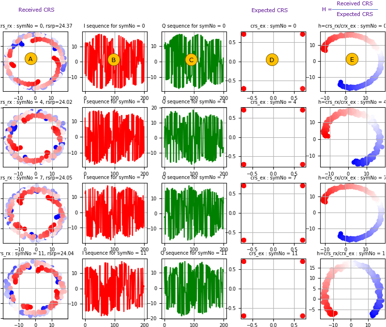
CRS channel estimation for symbols 0, 4, 7 and 11. (A) received CRS, (B) and (C) its in-phase and quadrature parts, (D) the expected CRS, (E) the channel estimate H = crs_rx / crs_ex.

The expected CRS in (D) are QPSK values at (+/-0.707, +/-0.707), with magnitude 1, so dividing by them mainly turns the phase. In (E), the estimate forms an arc of almost constant magnitude, and its phase changes steadily from one end of the band to the other. For port 0, the CRS sit every 6 subcarriers in symbols 0, 4, 7 and 11. Symbols 4 and 11 are shifted by 3 subcarriers against symbols 0 and 7 (36.211 v19.3.0 clause 6.10.1.2).

• 200 CRS per symbol : 2 per RB on 100 RB, port 0.
• H = crs_rx / crs_ex : a least-squares estimate at each CRS position.
• Symbols 4 and 11 shifted by 3 : against symbols 0 and 7.

H grid Construction

Now you got the channel coefficients for every resource elements where CRS is located. For the proper equalization for every resource elements in the resource grid, we need to figure out the channel coefficient for all other resource elements where there is no CRS.

A common way to get the channel coefficient for every resource elements is interpolate the CRS channel coefficient in frequency and time domain and construct a resource grid filled out with the estimated (interpolated) channel coefficient. The plot for the channel coefficient resource grid (H resource grid) would be something like this.

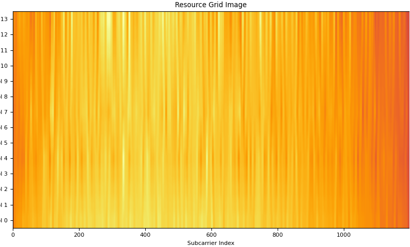
Magnitude of the interpolated H grid over 14 symbols and 1200 subcarriers.

The heatmap shown above may look fancy but would not give you much concrete meaning. Proabably plotting constellation for each OFDM symbol would give you more meaning / intuition of the channel as shown below.

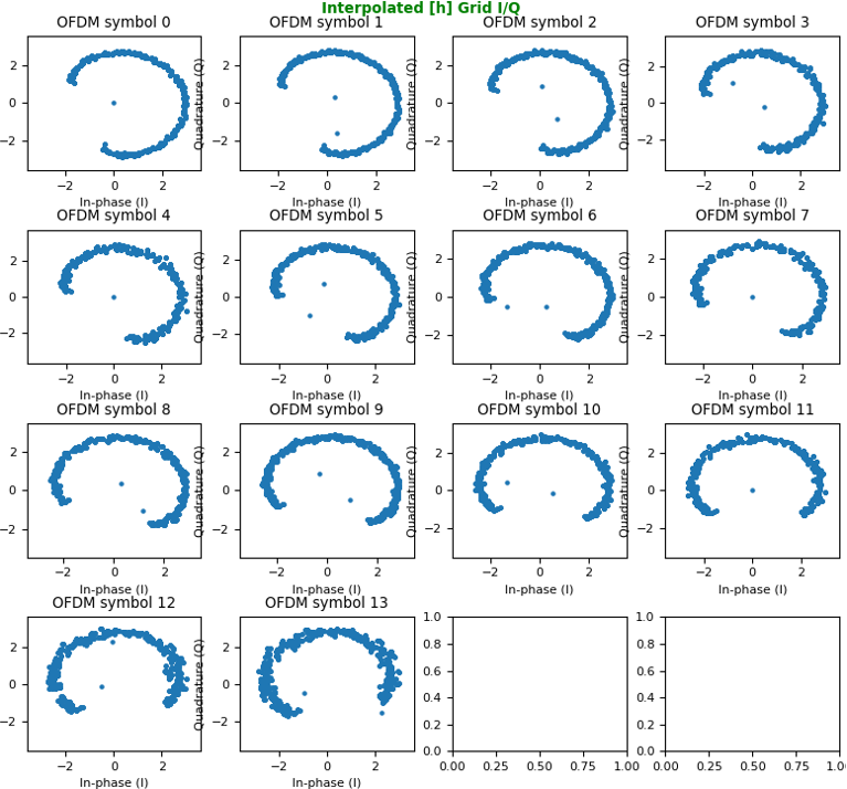
Interpolated H values per OFDM symbol. Each symbol forms the same arc of nearly constant magnitude.

Just for a little bit different aspect (view point) of the channel coefficient for each resource elements, I plotted amplutude and phase plot for the H resource grid as follows. The smallest index on horizontal axis corresponds to the subcarrier at the lowest frequency.

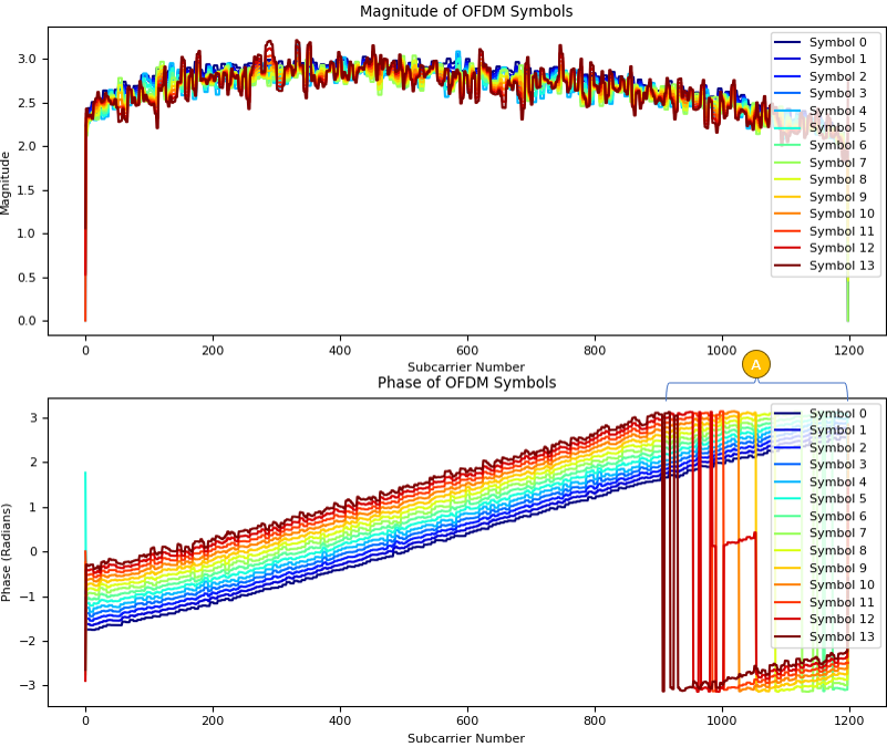
Magnitude and phase of H for each symbol. (A) marks where the phase passes +pi and wraps to -pi, which is a plotting effect.

The two plots above carry most of the information. The magnitude stays between about 2.3 and 3 across the band, so the cable gives a nearly flat channel. The phase rises almost linearly with the subcarrier index, by about 4.5 radians over 1200 subcarriers as read from the plot. A linear phase ramp across frequency is what a small timing offset of the FFT window produces. Here 4.5 / (2 x pi x 15 kHz x 1200) is about 40 ns, a little over one sample at 30.72 MHz.

The lines also step upward from symbol 0 to symbol 13, by roughly 1.4 radians over about 0.93 ms. That drift points to a residual frequency offset in the order of 240 Hz, left over from the constant-phase correction above.

Now let me show you how I got the full channel coefficient grid as shown above in step by step.

Step 1 :  Populate H values into an empty resource grid

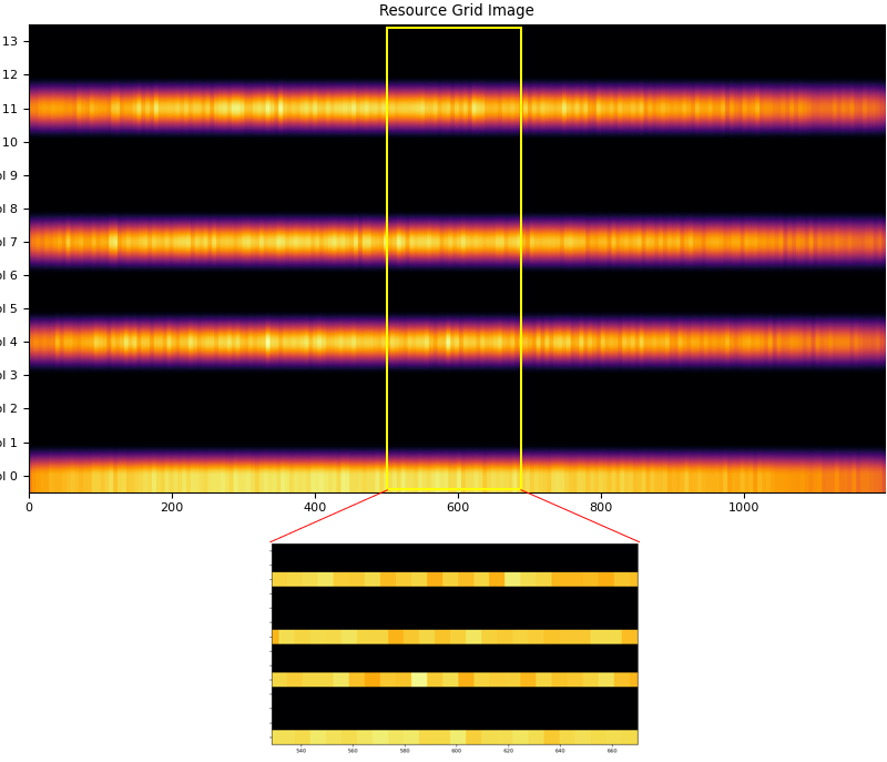
The first I did was to create an empty resource grid with same size as the data resource grid and the populate the H values for CRS at the proper CRS RE(Resource Element)s as shown below. You see that only CRS location has certain values (yellow / non-black) color and all other REs are empty (black)

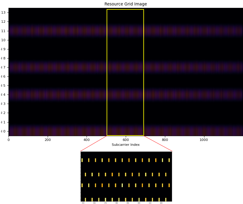
Step 1: H values at the CRS positions only. The zoom shows the 6-subcarrier spacing and the 3-subcarrier shift between symbols 0 and 4.

Step 2 :  Frequency Domain Interpolation

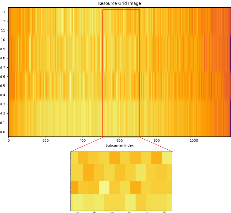
Now fill in the gaps only in frequency domain. You can do this by interpolating the values (complex value) along frequency domain. You may apply various ways of interpolation, but I did it just by moving average. The result of the frequency domain interpolation looks as follows.

Step 2: after frequency-domain interpolation, symbols 0, 4, 7 and 11 are filled across the band.

Step 3 :  Time Domain Interpolation

Now let's try to fill in the empty RE in time domain. Theoretically you can may use the same method as in frequency domain (moving average) or python package for the interpolation. But none of them work very good mainly because the number of points in time domain is too small. So I created my own interpolation function that can do the interpolation between only two end points. (NOTE : This is just for my own case, you may use different method of your own if you have any).

Here is broken down procedure of what I did

i) fill in symbol 1,2,3 by interpolating symbol 0 and 4 as end points

ii) fill in symbol 5,6  by interpolating symbol 4 and 7 as end points

iii) fill in symbol 8,9,10 by interpolating symbol 7 and 11 as end points

iv) fill in symbol 12, 13 by extrapolating symbol 9,10,11 (You may do this by interpolating the symbol 11 and symbol 0 of next subframe, but I did the extrapolation because I processed only one subframe with no next subframe).

Final result after all thse procedure, I get the resource grind as shown below.

Step 3: after time-domain interpolation, every RE of the subframe has an H value.

Linear interpolation between two CRS symbols works here because the channel changes slowly. The capture uses a cable, and the only change over time is the phase drift described above. With a moving UE, the channel can change within a slot, and receivers then use more CRS symbols or Wiener filtering across time and frequency. Symbols 12 and 13 lie after the last CRS symbol of the subframe, so they can only be extrapolated unless symbol 0 of the next subframe is available.

• Flat magnitude, linear phase : a nearly ideal cable channel with a small timing offset.
• Phase steps from symbol to symbol : a residual frequency offset of roughly 240 Hz.
• Frequency first, then time : symbols 12 and 13 need extrapolation.

Equalization

Equalization is the step where the channel estimate is finally used. Every data RE is divided by the H value at the same position, which undoes both the gain and the phase that the channel applied.

With the resource grid filled with channel coefficient for every resource element, now we are ready with equalizing every symbols (every resource elements) and recovering constellation.

The constellation before correction (i.e, before Equalization), it looks as below.

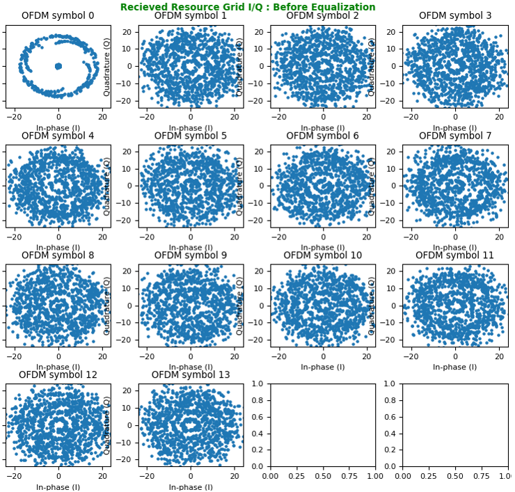
Received constellation of each OFDM symbol before equalization. The points form rings, because the channel phase differs from subcarrier to subcarrier.

Now let's compensate (equalize) the constellation with the channel coefficient. With the equalization, we can get the nicely aligned constellation as follows. The basic idea behind the equalization can be represented by a simple math as follows :

Corrected symbol (equalized symbol) = received symbol / channel coefficient

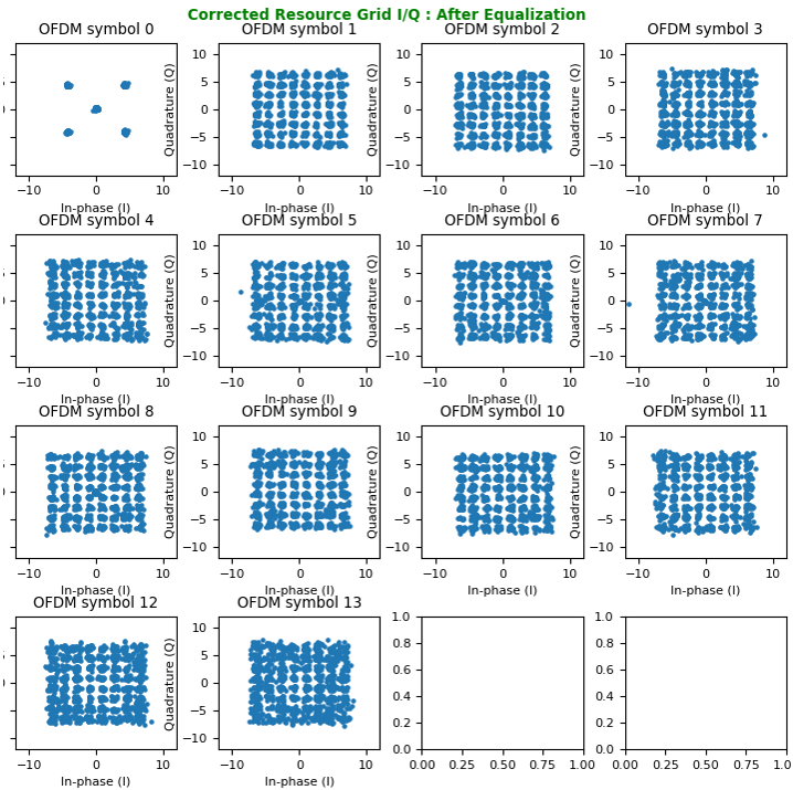
The same REs after equalization. Symbol 0 shows the QPSK control region and the unused REs at zero, and symbols 1 to 13 show a 64QAM grid.

This division is a zero-forcing equalizer for one antenna. It works well when noise is small, as in this cable capture. On a fading channel, dividing by a small H amplifies the noise on that subcarrier, and an MMSE equalizer, which weights the division by the noise level, performs better.

• Equalized symbol = received / H : zero forcing for SISO.
• 64QAM appears only after equalization : the rings before it come from the channel phase.
• SISO chain complete : PSS, CP removal, FFT, SSS, PCI, CRS, H grid, equalization.

MIMO 2x2

Decoding MIMO is much more complicated than SISO decoding in various aspect and there may be diverse variations of implementation. The overall procedure of my implementation is as follows.

i) Get the IQ data for 2 RX antenna (lets call them as iq_rx_0 and iq_rx_1 respectively)

ii) Detect PSS (detecting subframe boundary), Estimate Frequency Error and detect SSS for iq_rx_0 as I did for SISO

iii) Construct the Resource Grid for iq_rx_0 (let's call this as grid_rx_0)

iv) Construct the Resource Grid for iq_rx_1 with the same subframe boundary obtained from iq_rx_0 (let's call this as grid_rx_1)

v) Construct the H grid for 2x2 MIMO. In this case, I need to construct 4 H grid indicating channel coefficient for each path between 2 TX antenna and 2 RX antenna (let call them as h11, h21, h12, h22 respectively)

vi) perform time domain and frequency domain interpolation for h11,h21,h12,h22

vii) construct 2x2 H matrix for each resource elements from h11, h21, h12, h22 resource grid.

viii) Equalize grid_rx_0 and grid_rx_1 using the 2x2 H matrix

ix) Undo Precoding (I used 2x2 TM3 IQ signal. so I applied TM3 2x2 Precoding matrix for this step)

x) Undo Large CDD (I used 2x2 TM3 IQ signal. so I need to undo large CDD)

Resource Grid Construction - Antenna 0

The first step is to construct the resource grid for the signal captured by RX antenna 0 (iq_rx_0). This process is exactly same as I did for SISO.  Check out these for the details : PSS detection, Frequency Offset Estimation, CP (Cyclic Prefix) Removal, Resource Grid Reconstruction and the result resource grid is as follows.

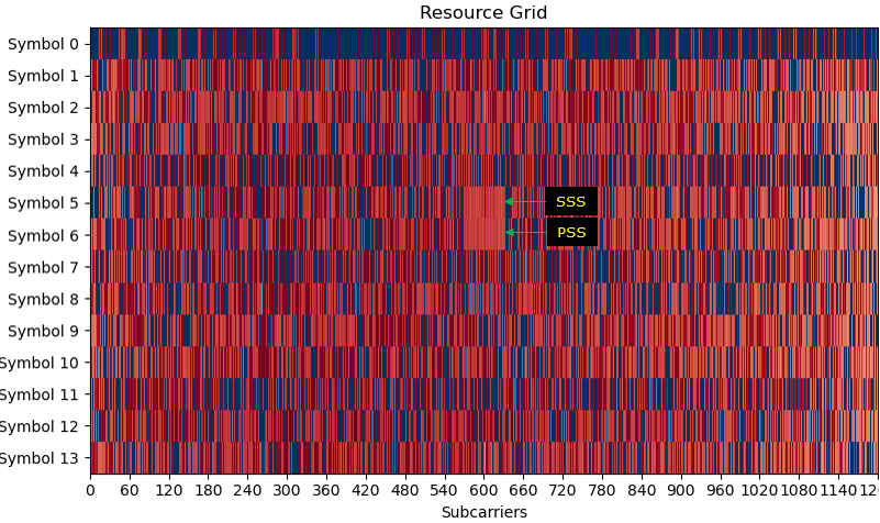
Resource grid from RX antenna 0, with the SSS in symbol 5 and the PSS in symbol 6.

Resource Grid Construction - Antenna 1

Now I have to construct the resource grid for the signal captured by RX antenna 1 (iq_rx_1), but I have to think of something at this point. As explained in SISO processing, there are a few steps to be done before the construction of the resource grid. The most important thing is to find 'start of a subframe (i.e, subframe boundary)' which is the sample position of the start of the subframe within the iq data(iq_rx_1). I can think of the two cases of finding the start of a subframe for iq_rx_1 as described below.

Case 1 : detecting the subframe boundary by performing PSS detection for iq_rx_1

Case 2 : Using the subframe boundary detected from iq_rx_0

You may use any of the two cases and other case if you have any better way. I used the case 2. If I use the case 1, the subframe boundary detected from iq_rx_1 and iq_rx_0 may not be the same. If there is even differences even by only one sample point, I may get completely wrong pair of data from the two RX antenna.

The resule of the construction of resource grid for iq_rx_1 based on Case 2 is shown below.

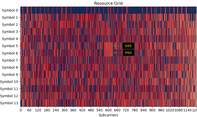
Resource grid from RX antenna 1, cut with the subframe boundary found on antenna 0.

H Grid Construction

Now I have to construct the channel matrix for this 2x2 MIMO case from the two resource grid that I obtained in previous step. In case of SISO, obtaining channel coefficient is relatively simple as shown here and here because the channel coefficient for each resource element is a scalar (complex valued scalar). However, for 2x2 MIMO we need to get an 2x2 matrix for channel coefficient for each resource element.

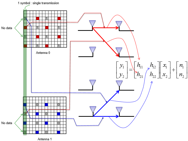
Channel matrix for 2x2 MIMO. The first index is the RX antenna and the second is the TX antenna, so h11 and h21 come from TX antenna 0.

The two TX ports can be measured separately because their CRS never overlap. On the REs where port 0 sends its CRS, port 1 sends nothing, and the other way round (36.211 v19.3.0 clause 6.10.1.2). So at a port 0 CRS position, RX antenna 0 sees h11 alone and RX antenna 1 sees h21 alone. The port 1 CRS give h12 and h22 in the same way.

The result of H resource grid at the position of CRS looks as bellow :  

NOTE : In this specific example, the I/Q data that I captured are from the conductive connection (i.e, TX antenna 0 is connected to RX antenna 0 and TX antenna 1 is connected to RX antenna 1 via RF cable. So theoretically h21 and h12 coefficient should be zero, but there can still be a small leakage, hence you see small values even for h21 and h12. However, the magnitude of h21 and h12 is much smaller (darker color in the plot) than h11, h22.

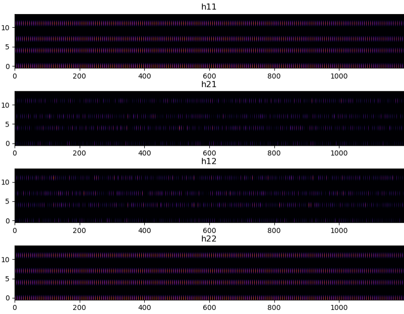
H at the CRS positions. The h11 and h22 grids are bright, and the h21 and h12 grids are dark, because the cable connects each TX antenna to one RX antenna.

Then I did the interpolation in frequency domain and time domain for h11,h12,h21,h22 and result are shown below. (The procedure for the implementation is same as explained in H grid construction for SISO processing.

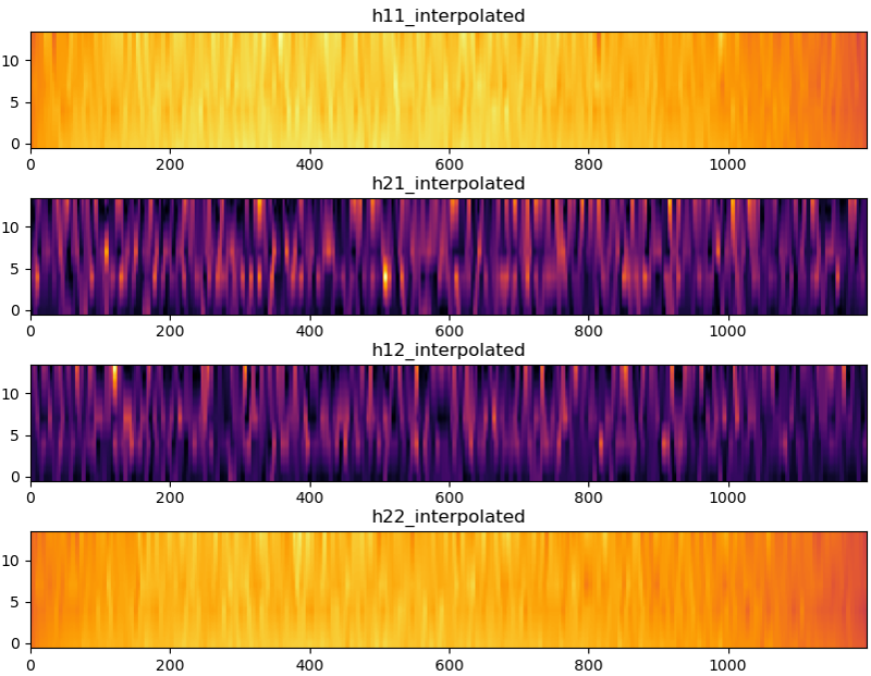
The four H grids after frequency-domain and time-domain interpolation.

Following is just another way of representing the interpolated H grid obtained above. I plotted each h coefficient at every resource elements for each ofdm symbol in the form of constellation. Here you would notice obviously the magnitude differences between h11,h22 and h21, h12.

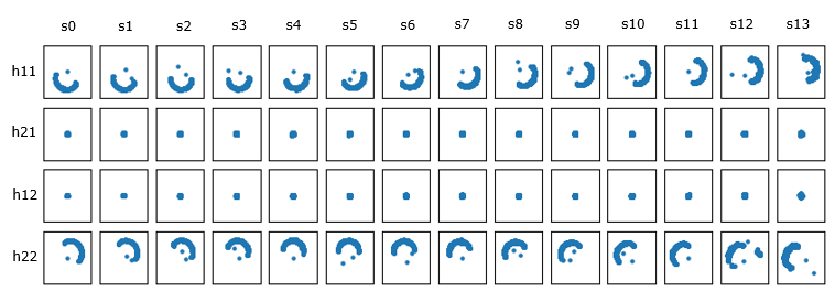
Interpolated H per symbol: arcs for h11 and h22, small clusters near zero for h21 and h12.

The arcs of h11 and h22 turn a little from s0 to s13. This is the same drift as in the SISO phase plot. Both antennas see it, because it comes from the frequency error of the capture, not from the cable.

Equalization

What I am going to do now is to equalize the received data with channel matrix obtained in previous step. The fundamental idea is same as done for SISO . The difference is that the channel coefficient for this case is 2x2 complex numbered matrix whereas it is complex numbered scalar for SISO.

NOTE : There are various methods of utilizing H matrix for equalization as shown in these notes , in this specfic example I am going to use direct inversion for simplicity.

Before performing Equalization, let me plot the received I/Q constellation for each OFDM symbol in constellation as shown below.

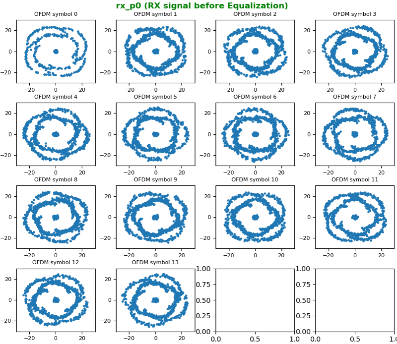
rx_p0, the grid of RX antenna 0, before equalization.

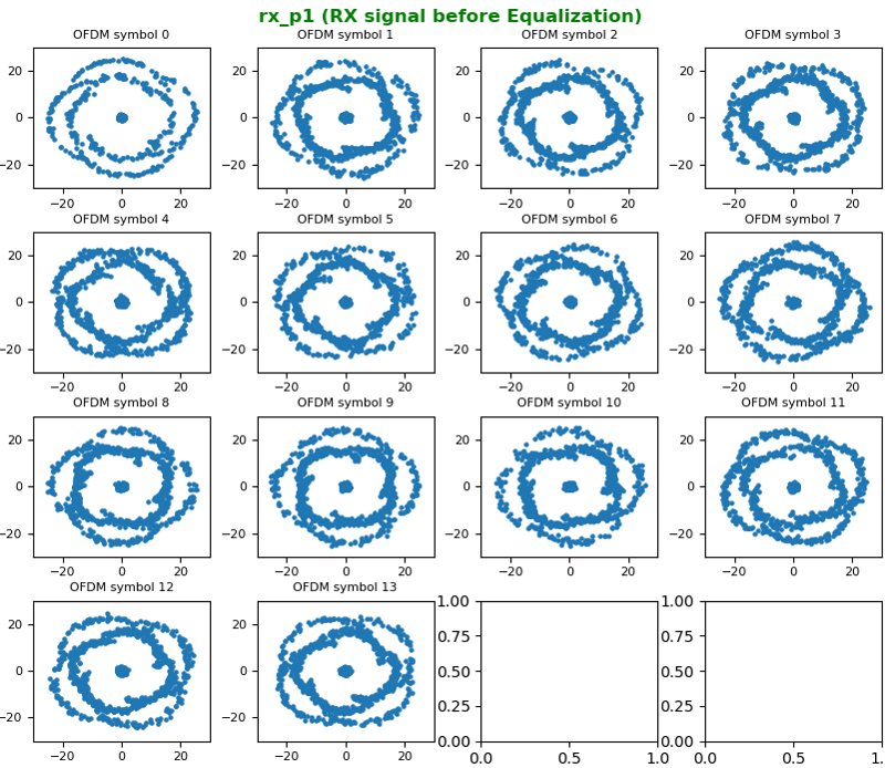
rx_p1, the grid of RX antenna 1, before equalization.

Then Equalize the received signal with H matrix and I got the constellation as shown below.

NOTE : The signal (PDSCH) that I captured for this example is QAM in LTE TM3 (Transmission Mode 3), but the constellation shown here does not look like QAM. Why ?  This will be explained in next section.

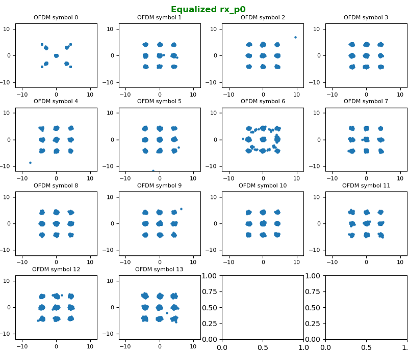
Equalized rx_p0: a 3 by 3 grid rather than a QPSK constellation.

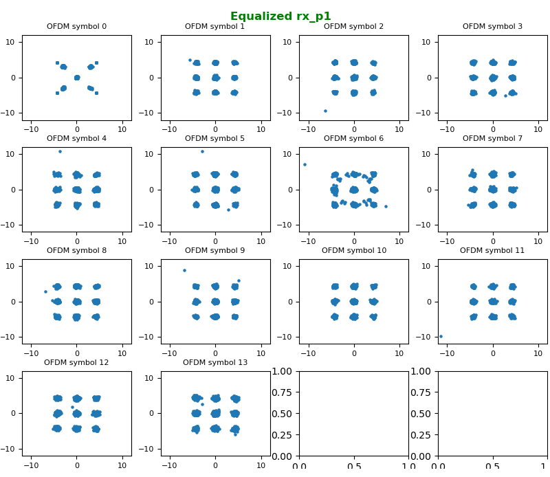
Equalized rx_p1: the same 3 by 3 grid.

Direct inversion computes x = H^-1 y for every RE, with y the pair of received values and H the 2 by 2 matrix at that RE. It recovers what the two TX antenna ports sent, not the layers themselves. With TM3, each port carries a mix of both layers, which is why the grid has 9 points: each value is a sum or a difference of two QPSK symbols. The next two sections remove that mix.

Precoding

In LTE, PDSCH gets precoded in various way depending on the type of TM (Transmission Mode) being used (If you are not familiar with TM, check out this note). The I/Q data used for this specific example is TM3 2x2 MIMO.

TM3 in LTE is done by two steps : first applied with precoding matrix W and then applied with Large CDD. This whole process is expressed in math form at the middle row shown below. Therefore, in decoding process all of this processes should be 'Undone'.

In encoding process(transmission process), U matrix is applied first, then D matrix and then W matrix. So in decoding process, this should be done in reverse order (i.e, undo W first, the D and then U). The mathematical meaning of 'Undo' is just to multiply the data with inverse of each matrix.

Precoding in 36.211: without CDD, with large-delay CDD and for transmit diversity, with the 2-port codebook of Table 6.3.4.2.3-1.

As explained above, in decoding process the first step is to undo precoding part, i.e, multiply the data with the inverse of W matrix. TM3 2x2 case, the codebook 0 is used. According to the codebook shown above, 2x2 codebook 0 is identify matrix normalized by sqrt(2). So the result of undoing W matrix is same as 'not doing anything' as shown below. You wouldn't see any difference from what you got in previous step.

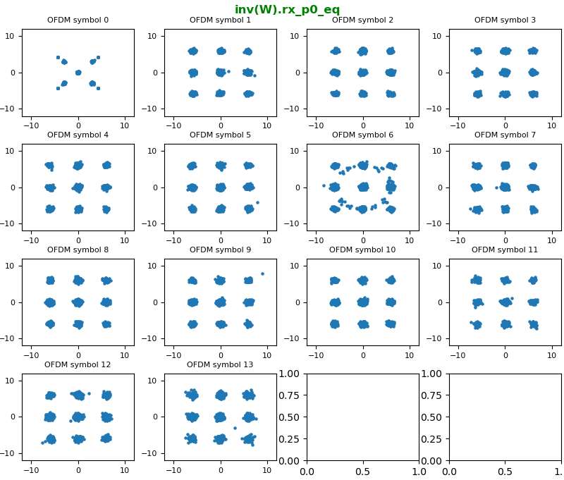
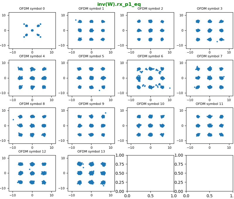
rx_p0 and rx_p1 after multiplying by the inverse of W. The grid grows by sqrt(2) and keeps its shape.

For large-delay CDD on 2 antenna ports, 36.211 v19.3.0 clause 6.3.4.2.2 fixes W(i) to precoder index 0 of Table 6.3.4.2.3-1. That matrix is the identity divided by sqrt(2), and its inverse is sqrt(2) times the identity. Undoing W therefore only scales the values, as the plots show: the 3 by 3 grid grows from about 4.3 to about 6. For 4 antenna ports, W(i) cycles through precoder indices 12 to 15, and this step would change the values.

Large CDD

Next step of undoing 'Precoding' for TM3 is to undo 'Large CDD'. The math process of Large CDD is illustrated below. So undoing Large CDD is to undo D matrix and then U matrix.

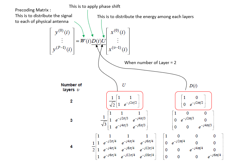
U and D(i) for large-delay CDD, from 36.211 Table 6.3.4.2.2-1.

Let's first undo D matrix for 2x2 and the result is shown below. Just by looking at the overall constellation, you would not notice any difference from the previous step. But if you look into the matrix itself in more detail, you would notice there is no differences in terms of rx_p0 constellation but there is phase delay of multiples of pi radian (meaning the rotating the constellation by multiples of pi radian). In constellation, if you rotate the point by multiples of 90 degree (pi/2 radian) you would not notice any big difference 

NOTE : If you are interested in math practice for this operation, Check out this ,this  and this note to get some intuitive understanding of this matrix. If you are seriously interested in this process, you need to have a good / concrete understandings on the math operation itself.

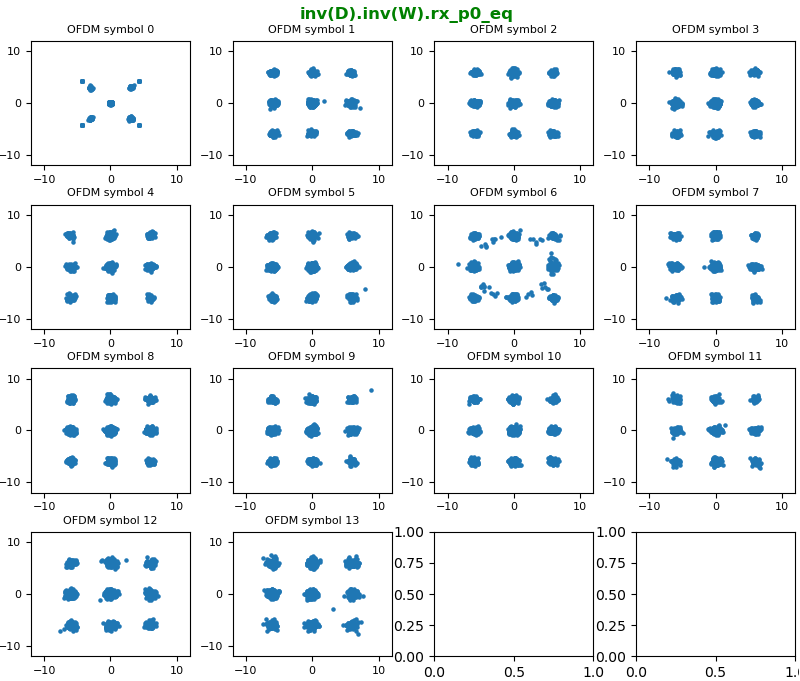
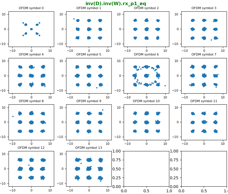
After undoing D(i). The constellation looks the same, because D(i) only flips the sign of layer 1 on every other symbol.

For 2 layers, D(i) = diag(1, e^{-j pi i}), so the second layer is multiplied by +1 and -1 in turn. The index i counts the PDSCH symbols of the layer in mapping order, not the subcarrier index. An implementation must therefore follow the RE order of the PDSCH mapping and skip the CRS and control REs. A sign flip maps the 3 by 3 grid onto itself, which is why the plots do not change.

Now let's undo the last part of Large CDD which is to undo U matrix. The result is as below. Now you see the QAM constellation as you expected.

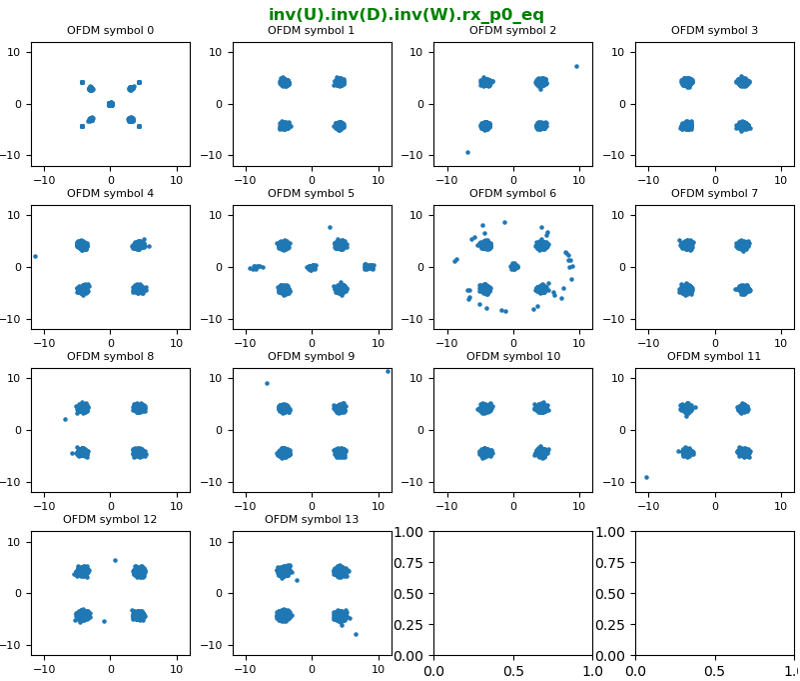
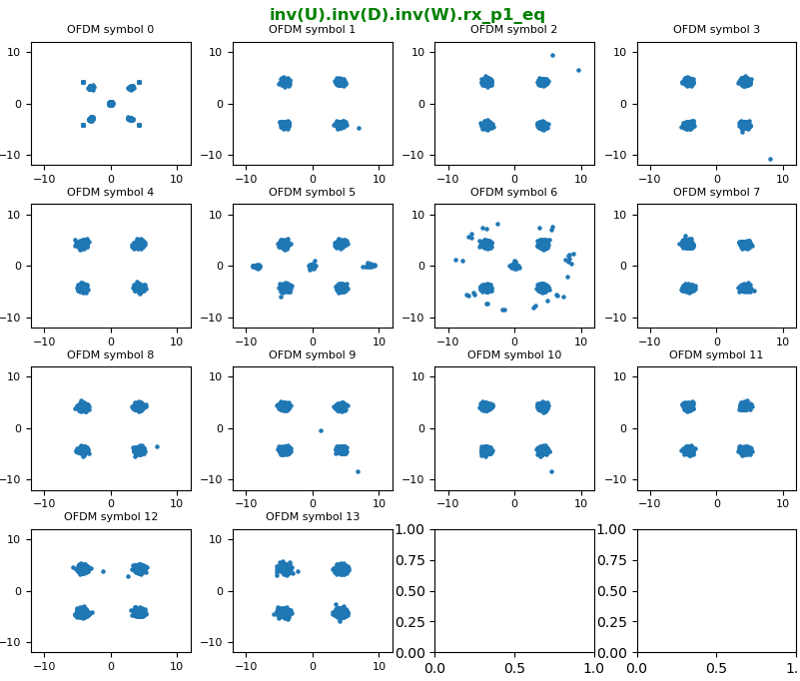
After undoing U: QPSK on both layers. The extra points in symbols 5 and 6 are the SSS and PSS REs, which are not precoded.

For 2 layers, U = (1/sqrt(2)) [1 1; 1 -1]. Its inverse adds and subtracts the two values, which separates the two QPSK layers and gives the 4-point constellation above. Symbol 0 is the same in every plot of this chain. It holds the control region, which is sent with transmit diversity, not large-delay CDD. In symbols 5 and 6, the SSS and PSS REs are not precoded, so the inverse matrices scatter them around the QPSK points.

• Equalization gives the antenna-port signals : a 3 by 3 grid with TM3.
• Undo W : only a sqrt(2) scaling on 2 ports.
• Undo D(i) : a sign flip of layer 1 on every other symbol.
• Undo U : sum and difference, giving QPSK on both layers.

Reference

[1] 3GPP TS 36.211 v19.3.0 - clauses 6.3.4.2.2 and 6.3.4.2.3, large-delay CDD and the codebook; clauses 6.10.1, 6.11 and 6.12, CRS, synchronization signals and OFDM baseband signal generation